تحسين تقدير الطاقة لنموذج شعرية فيرميوني باستخدام SQD
في هذا البرنامج التعليمي، ننفّذ نمط Qiskit يوضح كيفية المعالجة اللاحقة للعينات الكمية الضوضائية للعثور على تقريب لحالة الطاقة الأساسية لهاميلتونيان شعرية فيرميوني المعروف بنموذج أندرسون أحادي الشائبة. سنتبع نهج القطرنة الكمية المعتمدة على العينات لمعالجة العينات المأخوذة من مجموعة من حالات الأساس Krylov ذات 16 qubit عبر فترات زمنية متزايدة. تُحقَّق هذه الحالات على الجهاز الكمي باستخدام ترويتر للتطور الزمني. ولمراعاة أثر الضوضاء الكمية، تُستخدَم تقنية استعادة التهيئة. بافتراض حالة ابتدائية جيدة وندرة حالة الطاقة الأساسية، ثبت أن هذا النهج يتقارب بكفاءة.
يمكن وصف النمط في أربع خطوات:
- الخطوة 1: التعيين إلى مسألة كمية
- توليد مجموعة من حالات الأساس Krylov (أي دوائر التطور الزمني المرتّنة بطريقة تروتر) عبر فترات زمنية متزايدة لتقدير حالة الطاقة الأساسية
- الخطوة 2: تحسين المسألة
- نقل (Transpile) الدوائر إلى الـ Backend
- الخطوة 3: تنفيذ التجارب
- استخلاص العينات من الدوائر باستخدام بدائل
Sampler
- استخلاص العينات من الدوائر باستخدام بدائل
- الخطوة 4: المعالجة اللاحقة للنتائج
- حلقة استعادة التهيئة ذاتية الاتساق
- المعالجة اللاحقة لمجموعة العينات الكاملة من سلاسل البتات، باستخدام معرفة مسبقة بعدد الجسيمات ومتوسط إشغال المسار المحسوب في التكرار الأخير
- الإنشاء الاحتمالي لدفعات من العينات الفرعية من سلاسل البتات المستعادة
- إسقاط هاميلتونيان الشعرية الفيرميوني وقطرنته على كل فضاء جزئي من العينات
- حفظ أدنى طاقة للحالة الأساسية الموجودة عبر جميع الدفعات وتحديث متوسط إشغال المسار
- حلقة استعادة التهيئة ذاتية الاتساق
الخطوة 1: تعيين المسألة إلى دائرة كمية
أولاً، سننشئ هاميلتونيَّي الجسم الواحد والجسمين اللذين يصفان نموذج أندرسون أحادي الشائبة أحادي البُعد (SIAM) مع 7 مواقع حمّام (8 إلكترونات في 8 مسارات). يُستخدم هذا النموذج لوصف الشوائب المغناطيسية المضمّنة في المعادن.
ثم سننشئ دوائر تروتر ذات 16 qubit المستخدمة لتوليد الفضاء الجزئي الكمي Krylov.
# Added by doQumentation — required packages for this notebook
!pip install -q ffsim matplotlib numpy qiskit qiskit-addon-sqd qiskit-ibm-runtime scipy
import numpy as np

n_bath = 7  # number of bath sites

V = 1  # hybridization amplitude
t = 1  # bath hopping amplitude
U = 10  # Impurity onsite repulsion
eps = -U / 2  # Chemical potential for the impurity

# Place the impurity on the first qubit
impurity_index = 0

# One body matrix elements in the "position" basis
h1e = -t * np.diag(np.ones(n_bath), k=1) - t * np.diag(np.ones(n_bath), k=-1)
h1e[impurity_index, impurity_index + 1] = -V
h1e[impurity_index + 1, impurity_index] = -V
h1e[impurity_index, impurity_index] = eps

# Two body matrix elements in the "position" basis
h2e = np.zeros((n_bath + 1, n_bath + 1, n_bath + 1, n_bath + 1))
h2e[impurity_index, impurity_index, impurity_index, impurity_index] = U
بعد ذلك، سنولّد الفضاء الجزئي الكمي Krylov بمجموعة من الدوائر الكمية المرتّنة بطريقة تروتر. ننشئ هنا مساعدات لتوليد الحالة الابتدائية (المرجعية) وكذلك التطور الزمني للجزأين أحادي الجسم وثنائي الجسم من الهاميلتوني. للاطلاع على وصف أكثر تفصيلاً لهذا النموذج وكيفية تصميم الدوائر، يُرجى الرجوع إلى الورقة البحثية.
import ffsim
import scipy
from qiskit import QuantumCircuit, QuantumRegister
from qiskit.circuit.library import CPhaseGate, XGate, XXPlusYYGate

n_modes = n_bath + 1
nelec = (n_modes // 2, n_modes // 2)

dt = 0.2
Utar = scipy.linalg.expm(-1j * dt * h1e)

# The reference state
def initial_state(q_circuit, norb, nocc):
    """Prepare an initial state."""
    for i in range(nocc):
        q_circuit.append(XGate(), [i])
        q_circuit.append(XGate(), [norb + i])
    rot = XXPlusYYGate(np.pi / 2, -np.pi / 2)

    for i in range(3):
        for j in range(nocc - i - 1, nocc + i, 2):
            q_circuit.append(rot, [j, j + 1])
            q_circuit.append(rot, [norb + j, norb + j + 1])
    q_circuit.append(rot, [j + 1, j + 2])
    q_circuit.append(rot, [norb + j + 1, norb + j + 2])

# The one-body time evolution
free_fermion_evolution = ffsim.qiskit.OrbitalRotationJW(n_modes, Utar)

# The two-body time evolution
def append_diagonal_evolution(dt, U, impurity_qubit, num_orb, q_circuit):
    """Append two-body time evolution to a quantum circuit."""
    if U != 0:
        q_circuit.append(
            CPhaseGate(-dt / 2 * U),
            [impurity_qubit, impurity_qubit + num_orb],
        )
يتم توليد d من الحالات المتطورة زمنياً التي تحدّد الفضاء الجزئي الكمي Krylov. اخترنا هنا d=8. يتقارب الخطأ الناتج عن أخذ عينات من حالات أساس Krylov مع زيادة d. لاحظ أن خصائص مثيل هذه المسألة تسمح بتجميع فعّال لتطور الجسم الواحد باستخدام OrbitalRotationJW؛ غير أنه بوجه عام، يمكن استخدام PauliEvolutionGate في Qiskit لتنفيذ التطور الزمني المرتّن بطريقة تروتر للهاميلتوني الكامل.
# Generate the initial state
qubits = QuantumRegister(2 * n_modes, name="q")
init_state = QuantumCircuit(qubits)
initial_state(init_state, n_modes, n_modes // 2)
init_state.draw("mpl", scale=0.4, fold=-1)

d = 8  # Number of Krylov basis states
circuits = []
for i in range(d):
    circ = init_state.copy()
    circuits.append(circ)
    for _ in range(i):
        append_diagonal_evolution(dt, U, impurity_index, n_modes, circ)
        circ.append(free_fermion_evolution, qubits)
        append_diagonal_evolution(dt, U, impurity_index, n_modes, circ)
    circ.measure_all()
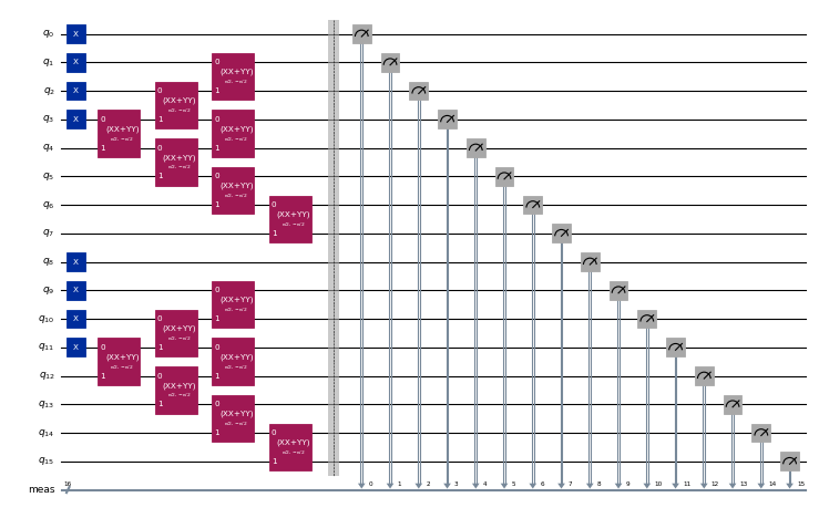
circuits[0].draw("mpl", scale=0.4, fold=-1)
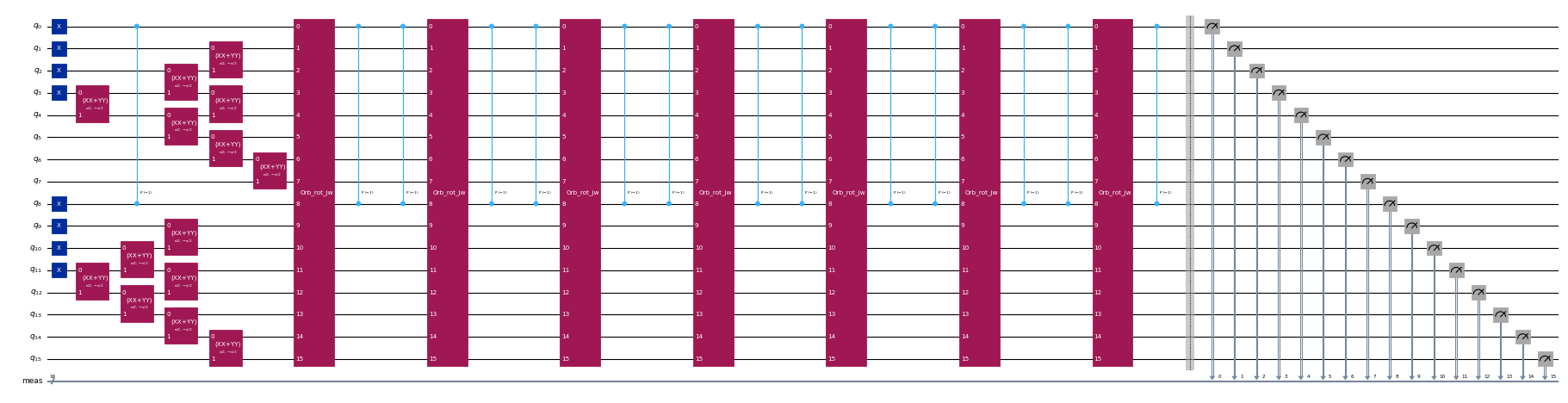
circuits[-1].draw("mpl", scale=0.4, fold=-1)
الخطوة 2: تحسين المسألة
بعد إنشاء الدوائر المرتّنة بطريقة تروتر، سنحسّنها لأجهزة العتاد المستهدفة. نحتاج إلى اختيار جهاز العتاد قبل التحسين. سنستخدم Backend وهمياً بسعة 127 qubit من qiskit_ibm_runtime لمحاكاة جهاز حقيقي. للتشغيل على وحدة معالجة كمية حقيقية، استبدل فقط الـ Backend الوهمي بـ Backend حقيقي. اطلع على وثائق Qiskit IBM Runtime لمزيد من المعلومات.
from qiskit_ibm_runtime.fake_provider.backends import FakeSherbrooke

backend = FakeSherbrooke()
بعد ذلك، سننقل (Transpile) الدوائر إلى الـ Backend المستهدف باستخدام Qiskit.
from qiskit.transpiler import generate_preset_pass_manager

# The circuit needs to be transpiled to the AerSimulator target
pass_manager = generate_preset_pass_manager(optimization_level=3, backend=backend)
isa_circuits = pass_manager.run(circuits)
الخطوة 3: تنفيذ التجارب
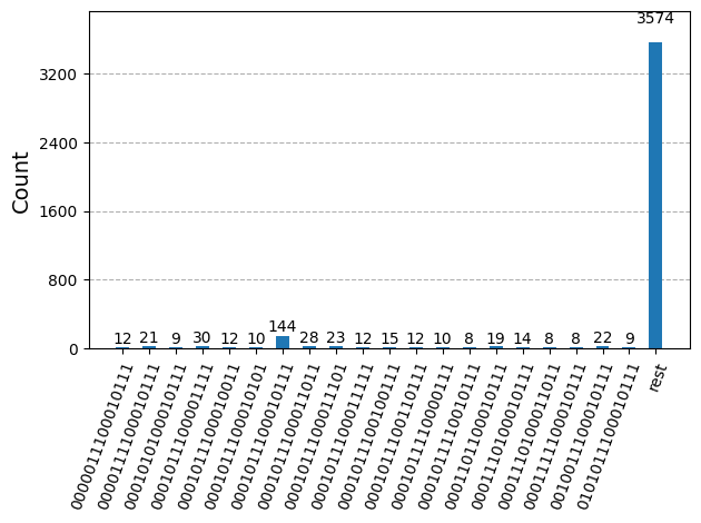
بعد تحسين الدوائر لتنفيذها على العتاد، أصبحنا جاهزين لتشغيلها على العتاد المستهدف وجمع العينات لتقدير طاقة الحالة الأساسية. نستخدم هنا SamplerV2 من qiskit-ibm-runtime لمحاكاة عينات ضوضائية مأخوذة من الـ Backend ibm_sherbrooke. ثم ندمج الأعداد من كل حالات الأساس Krylov في قاموس أعداد واحد ونرسم أعلى 20 سلسلة بتات الأكثر شيوعاً في العينات.
ملاحظة: Qiskit Aer مطلوب لمحاكاة العينات من الدوائر المنقولة.
from qiskit.primitives import BitArray
from qiskit.visualization import plot_histogram
from qiskit_ibm_runtime import SamplerV2 as Sampler

# Sample from the circuits
noisy_sampler = Sampler(backend, options={"simulator": {"seed_simulator": 24}})
job = noisy_sampler.run(isa_circuits, shots=500)

# Combine the counts from the individual Trotter circuits
bit_array = BitArray.concatenate_shots([result.data.meas for result in job.result()])

plot_histogram(bit_array.get_counts(), number_to_keep=20)
الخطوة 4: المعالجة اللاحقة للنتائج
الآن، نُشغّل خوارزمية SQD باستخدام الدالة diagonalize_fermionic_hamiltonian. راجع وثائق API للاطلاع على شرح وسائط هذه الدالة.
from qiskit_addon_sqd.fermion import SCIResult, diagonalize_fermionic_hamiltonian

# List to capture intermediate results
result_history = []

def callback(results: list[SCIResult]):
    result_history.append(results)
    iteration = len(result_history)
    print(f"Iteration {iteration}")
    for i, result in enumerate(results):
        print(f"\tSubsample {i}")
        print(f"\t\tEnergy: {result.energy}")
        print(f"\t\tSubspace dimension: {np.prod(result.sci_state.amplitudes.shape)}")

rng = np.random.default_rng(24)
result = diagonalize_fermionic_hamiltonian(
    h1e,
    h2e,
    bit_array,
    samples_per_batch=300,
    norb=n_modes,
    nelec=nelec,
    num_batches=3,
    max_iterations=10,
    symmetrize_spin=True,
    callback=callback,
    seed=rng,
)
Iteration 1
	Subsample 0
		Energy: -13.257128325607997
		Subspace dimension: 3969
	Subsample 1
		Energy: -13.257128325607997
		Subspace dimension: 3969
	Subsample 2
		Energy: -13.257128325607997
		Subspace dimension: 3969
Iteration 2
	Subsample 0
		Energy: -13.319666127542039
		Subspace dimension: 4096
	Subsample 1
		Energy: -13.420534292304595
		Subspace dimension: 4624
	Subsample 2
		Energy: -9.136171594591085
		Subspace dimension: 4624
Iteration 3
	Subsample 0
		Energy: -13.422491814612833
		Subspace dimension: 4900
	Subsample 1
		Energy: -13.422491814612833
		Subspace dimension: 4900
	Subsample 2
		Energy: -13.422491814612833
		Subspace dimension: 4900
Iteration 4
	Subsample 0
		Energy: -13.422491814612833
		Subspace dimension: 4900
	Subsample 1
		Energy: -13.422491814612833
		Subspace dimension: 4900
	Subsample 2
		Energy: -13.422491814612833
		Subspace dimension: 4900
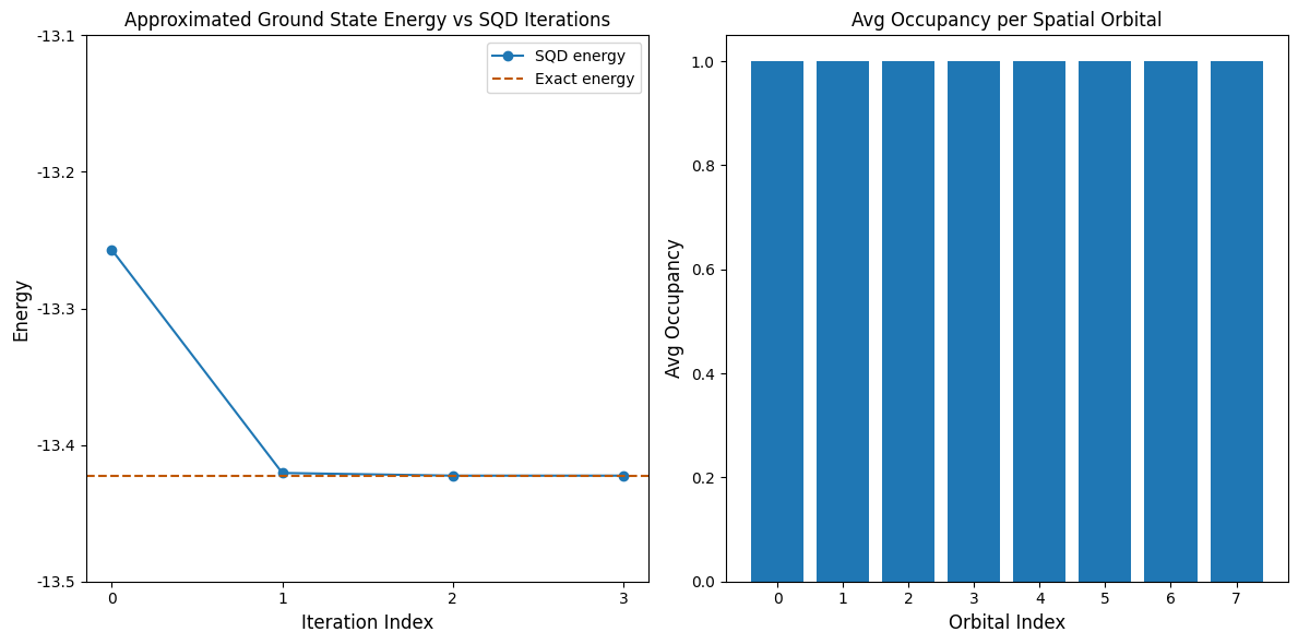
الآن، نرسم النتائج. يُظهر الرسم الأول أنه بعد عدد قليل من التكرارات، نحصل على طاقة الحالة الأساسية الدقيقة.
هذا المثال صغير بما يكفي لاستكشاف فضاء هيلبرت الكامل، كما يتضح من العبارات المطبوعة أعلاه. تذكّر أن فضاء هيلبرت الكامل له بُعد (num_orbitals choose nelec_a) * (num_orbitals choose nelec_b). لذا بالنسبة لهذه المسألة: (8 choose 4)**2 = 4900. تزداد أبعاد الفضاء الجزئي بسبب استعادة التهيئة المعزّزة، وأيضاً بسبب أن خوارزمية SQD تحمل التهيئات المهمة من تكرار إلى آخر. بحلول التكرار الأخير، نُجري القطرنة في فضاء هيلبرت الكامل.
يُظهر الرسم الثاني متوسط إشغال كل مسار مكاني عبر حلول جميع الدفعات. نرى أنه باحتمال كبير، يحتوي كل مسار على إلكترون واحد.
import matplotlib.pyplot as plt

exact_energy = -13.422491814605827
min_es = [min(result, key=lambda res: res.energy).energy for result in result_history]
min_id, min_e = min(enumerate(min_es), key=lambda x: x[1])

# Data for energies plot
x1 = range(len(result_history))
yt1 = list(np.arange(-13.5, -13.1, 0.1))
ytl = [f"{i:.1f}" for i in yt1]

# Data for avg spatial orbital occupancy
y2 = np.sum(result.orbital_occupancies, axis=0)
x2 = range(len(y2))

fig, axs = plt.subplots(1, 2, figsize=(12, 6))

# Plot energies
axs[0].plot(x1, min_es, label="SQD energy", marker="o")
axs[0].set_xticks(x1)
axs[0].set_xticklabels(x1)
axs[0].set_yticks(yt1)
axs[0].set_yticklabels(ytl)
axs[0].axhline(y=exact_energy, color="#BF5700", linestyle="--", label="Exact energy")
axs[0].set_title("Approximated Ground State Energy vs SQD Iterations")
axs[0].set_xlabel("Iteration Index", fontdict={"fontsize": 12})
axs[0].set_ylabel("Energy", fontdict={"fontsize": 12})
axs[0].legend()

# Plot orbital occupancy
axs[1].bar(x2, y2, width=0.8)
axs[1].set_xticks(x2)
axs[1].set_xticklabels(x2)
axs[1].set_title("Avg Occupancy per Spatial Orbital")
axs[1].set_xlabel("Orbital Index", fontdict={"fontsize": 12})
axs[1].set_ylabel("Avg Occupancy", fontdict={"fontsize": 12})

print(f"Exact energy: {exact_energy:.5f}")
print(f"SQD energy: {min_e:.5f}")
print(f"Absolute error: {abs(min_e - exact_energy):.5f}")
plt.tight_layout()
plt.show()
Exact energy: -13.42249
SQD energy: -13.42249
Absolute error: 0.00000