البتات الكمومية والبوابات والدوائر

ملاحظة

Kifumi Numata (19 Apr 2024)

اضغط هنا لتنزيل نسخة PDF من المحاضرة الأصلية. لاحظ أن بعض مقاطع الكود قد تكون قديمة لأنها صور ثابتة.

وقت وحدة المعالجة الكمومية التقريبي لتشغيل هذه التجربة هو 5 ثوانٍ.

1. المقدمة

البتات والبوابات والدوائر هي اللبنات الأساسية للحوسبة الكمومية. ستتعلم الحوسبة الكمومية باستخدام نموذج الدائرة القائم على البتات الكمومية والبوابات، وستراجع أيضاً مفاهيم التراكب والقياس والتشابك.

في هذا الدرس ستتعلم:

• بوابات الكيوبت الواحد
• كرة بلوخ
• التراكب
• القياس
• بوابات الكيوبتين وحالة التشابك

في نهاية هذه المحاضرة، ستتعرف على عمق الدائرة، وهو أمر جوهري للحوسبة الكمومية على نطاق المنفعة.

2. الحوسبة كرسم بياني

عند التعامل مع الكيوبتات أو البتات، نحتاج إلى معالجتها لتحويل المدخلات إلى المخرجات المطلوبة. في أبسط البرامج التي تحتوي على بتات قليلة جداً، يكون من المفيد تمثيل هذه العملية في رسم بياني يُعرف بـ رسم الدائرة.

الشكل في الأسفل على اليسار هو مثال على دائرة كلاسيكية، والشكل في الأسفل على اليمين هو مثال على دائرة كمومية. في كلتا الحالتين، المدخلات على اليسار والمخرجات على اليمين، بينما تُمثَّل العمليات برموز. وتُسمى هذه الرموز "بوابات"، في الغالب لأسباب تاريخية.

3. بوابة الكيوبت الواحد الكمومية

3.1 الحالة الكمومية وكرة بلوخ

تُمثَّل حالة الكيوبت كتراكب لـ $|0\rangle$ و $|1\rangle$. وتُعبَّر عن حالة كمومية اعتباطية بالصيغة:

$$|\psi\rangle =\alpha|0\rangle+ \beta|1\rangle$$

حيث $\alpha$ و $\beta$ أعداد مركبة تحقق $|\alpha|^2+|\beta|^2=1$.

$|0\rangle$ و $|1\rangle$ هما متجهان في الفضاء المتجهي المركب ثنائي الأبعاد:

$$|0\rangle = \begin{pmatrix} 1 \\0 \end{pmatrix}, |1\rangle = \begin{pmatrix} 0\\1 \end{pmatrix}$$

وبناءً على ذلك، تُمثَّل أي حالة كمومية اعتباطية أيضاً بالصيغة:

$$|\psi\rangle = \alpha\begin{pmatrix} 1 \\ 0 \end{pmatrix} + \beta\begin{pmatrix}0\\ 1 \end{pmatrix} = \begin{pmatrix} \alpha \\ \beta \end{pmatrix}$$

من هذا يتضح أن حالة البت الكمومي هي متجه وحدوي في فضاء الضرب الداخلي المركب ثنائي الأبعاد بأساس متعامد معياري هو $|0\rangle$ و $|1\rangle$، وهو مُعيَّر إلى 1.

$$\langle\psi|\psi\rangle = \begin{pmatrix} \alpha^* & \beta^* \end{pmatrix} \begin{pmatrix} \alpha \\ \beta \end{pmatrix} = 1$$

|\psi\rangle =\begin\{pmatrix\} \alpha \\ \beta \end\{pmatrix\} يُسمى أيضاً متجه الحالة (statevector).

كما يمكن تمثيل حالة الكيوبت الواحد بالصيغة:

$$|\psi\rangle =\cos\frac{\theta}{2}|0\rangle+e^{i\varphi}\sin\frac{\theta}{2}|1\rangle =\left( \begin{pmatrix} \cos\frac{\theta}{2}\\ e^{i\varphi}\sin\frac{\theta}{2} \end{pmatrix}\right)$$

حيث $\theta$ و $\varphi$ هما زاويا كرة بلوخ الموضحة في الشكل التالي.

في خلايا الكود التالية، سنبني الحسابات الأساسية خطوة بخطوة باستخدام Qiskit. سننشئ دائرة فارغة ثم نضيف العمليات الكمومية، ونناقش البوابات ونتخيل تأثيراتها أثناء التطبيق. يمكنك تشغيل الخلية بالضغط على "Shift" + "Enter". ابدأ باستيراد المكتبات أولاً.

# Added by doQumentation — required packages for this notebook
!pip install -q qiskit qiskit-aer qiskit-ibm-runtime

# Import the qiskit library
from qiskit import QuantumCircuit
from qiskit_aer import AerSimulator
from qiskit.quantum_info import Statevector
from qiskit.visualization import plot_bloch_multivector
from qiskit_ibm_runtime import Sampler
from qiskit.transpiler.preset_passmanagers import generate_preset_pass_manager
from qiskit.visualization import plot_histogram

إعداد الدائرة الكمومية

سننشئ دائرة من كيوبت واحد ونرسمها.

# Create the single-qubit quantum circuit
qc = QuantumCircuit(1)

# Draw the circuit
qc.draw("mpl")

بوابة X

بوابة X هي دوران بمقدار $\pi$ حول محور $x$ في كرة بلوخ. تطبيق بوابة X على $|0\rangle$ ينتج $|1\rangle$، وتطبيقها على $|1\rangle$ ينتج $|0\rangle$، لذا فهي عملية مشابهة لبوابة NOT الكلاسيكية، وتُعرف أيضاً بقلب البت. التمثيل المصفوفي لبوابة X هو:

$$X = \begin{pmatrix} 0 & 1 \\ 1 & 0 \\ \end{pmatrix}$$

qc = QuantumCircuit(1)  # Prepare the single-qubit quantum circuit

# Apply a X gate to qubit 0
qc.x(0)

# Draw the circuit
qc.draw("mpl")

في IBM Quantum®، الحالة الأولية تُضبط على $|0\rangle$، لذا فإن الدائرة الكمومية أعلاه بالتمثيل المصفوفي هي:

$$X|0\rangle= \begin{pmatrix} 0 & 1 \\ 1 & 0 \end{pmatrix} \begin{pmatrix} 1 \\ 0 \end{pmatrix} =\begin{pmatrix} 0 \\ 1 \end{pmatrix} = |1\rangle$$

لننفّذ الآن هذه الدائرة باستخدام محاكي متجه الحالة.

# See the statevector
out_vector = Statevector(qc)
print(out_vector)

# Draw a Bloch sphere
plot_bloch_multivector(out_vector)

Statevector([0.+0.j, 1.+0.j],
            dims=(2,))

يُعرض المتجه العمودي كمتجه صفي، مع الأعداد المركبة (الجزء التخيلي يُشار إليه بـ $j$).

بوابة H

بوابة هادامارد هي دوران بمقدار $\pi$ حول محور يقع في منتصف المسافة بين محوري $x$ و $z$ على كرة بلوخ. تطبيق بوابة H على $|0\rangle$ ينتج حالة تراكب مثل $\frac{|0\rangle + |1\rangle}{\sqrt{2}}$. التمثيل المصفوفي لبوابة H هو:

$$H = \frac{1}{\sqrt{2}}\begin{pmatrix} 1 & 1 \\ 1 & -1 \\ \end{pmatrix}$$

qc = QuantumCircuit(1)  # Create the single-qubit quantum circuit

# Apply an Hadamard gate to qubit 0
qc.h(0)

# Draw the circuit
qc.draw(output="mpl")

# See the statevector
out_vector = Statevector(qc)
print(out_vector)

# Draw a Bloch sphere
plot_bloch_multivector(out_vector)

Statevector([0.70710678+0.j, 0.70710678+0.j],
            dims=(2,))

هذا هو:

$$H|0\rangle= \frac{1}{\sqrt{2}} \begin{pmatrix} 1 & 1 \\ 1 & -1 \end{pmatrix} \begin{pmatrix} 1 \\0 \end{pmatrix} =\frac{1}{\sqrt{2}}\begin{pmatrix} 1 \\ 1 \end{pmatrix} =\begin{pmatrix} 0.707 \\ 0.707 \end{pmatrix} =\frac{1}{\sqrt{2}}(|0\rangle+|1\rangle)$$

حالة التراكب هذه شائعة ومهمة جداً لدرجة أنه أُعطيت رمزاً خاصاً بها:

$$|+\rangle \equiv \frac{1}{\sqrt{2}}(|0\rangle+|1\rangle).$$

بتطبيق البوابة $H$ على $|0\rangle$، أنشأنا تراكباً بين $|0\rangle$ و $|1\rangle$ بحيث يعطي القياس في الأساس الحسابي (على طول المحور z في صورة كرة بلوخ) كل حالة باحتمالية متساوية.

حالة $|-\rangle$

ربما خمّنت أن هناك حالة مقابلة $|-\rangle$:

$$|-\rangle \equiv \frac{|0\rangle -|1\rangle}{\sqrt{2}}.$$

لإنشاء هذه الحالة، طبّق أولاً بوابة X للحصول على $|1\rangle$، ثم طبّق بوابة H.

qc = QuantumCircuit(1)  # Create the single-qubit quantum circuit

# Apply a X gate to qubit 0
qc.x(0)

# Apply an Hadamard gate to qubit 0
qc.h(0)

# draw the circuit
qc.draw(output="mpl")

# See the statevector
out_vector = Statevector(qc)
print(out_vector)

# Draw a Bloch sphere
plot_bloch_multivector(out_vector)

Statevector([ 0.70710678+0.j, -0.70710678+0.j],
            dims=(2,))

هذا هو:

$$H|1\rangle= \frac{1}{\sqrt{2}} \begin{pmatrix} 1 & 1 \\\ 1 & -1 \end{pmatrix} \begin{pmatrix} 0 \\\ 1 \end{pmatrix} =\frac{1}{\sqrt{2}}\begin{pmatrix} 1 \\\ -1 \end{pmatrix} =\begin{pmatrix} 0.707 \\\ -0.707 \end{pmatrix} =\frac{1}{\sqrt{2}}(|0\rangle-|1\rangle) = |-\rangle$$

تطبيق البوابة $H$ على $|1\rangle$ ينتج تراكباً متساوياً بين $|0\rangle$ و $|1\rangle$، لكن إشارة $|1\rangle$ تكون سالبة.

3.2 الحالة الكمية لـ Qubit الواحد والتطور الوحداني

إجراءات جميع البوابات التي رأيناها حتى الآن كانت وحدانية (unitary)، وهذا يعني أنه يمكن تمثيلها بمؤثر وحداني. بمعنى آخر، يمكن الحصول على حالة الإخراج بتطبيق مصفوفة وحدانية على الحالة الابتدائية:

$$|\psi^{'}\rangle = U|\psi\rangle$$

المصفوفة الوحدانية هي مصفوفة تحقق الشرط

$$U^{\dagger}U =U U^{\dagger} = I.$$

من منظور عمليات الحاسوب الكمي، نقول إن تطبيق بوابة كمية على الـ qubit يُطوّر الحالة الكمية. ومن أبرز بوابات الـ qubit الواحد ما يلي.

بوابات باولي:

$$X = \begin{pmatrix} 0 & 1 \\ 1 & 0 \\ \end{pmatrix} = |0\rangle \langle 1|+|1\rangle \langle 0|$$ $$Y = \begin{pmatrix} 0 & -i \\ i & 0 \\ \end{pmatrix} = -i|0\rangle \langle 1|+i|1\rangle \langle 0|$$ $$Z = \begin{pmatrix} 1 & 0 \\ 0 & -1 \\ \end{pmatrix} = |0\rangle \langle 0|-|1\rangle \langle 1|$$

حيث يُحسب الضرب الخارجي كما يلي:

$$|0\rangle \langle 0|= \begin{bmatrix} 1 \\ 0 \end{bmatrix} \begin{bmatrix} 1 & 0 \end{bmatrix} =\begin{bmatrix} 1 & 0 \\ 0 & 0 \\ \end{bmatrix}, \quad |1\rangle \langle 0|= \begin{bmatrix} 0 \\ 1 \end{bmatrix} \begin{bmatrix} 1 & 0 \end{bmatrix} =\begin{bmatrix} 0 & 0 \\ 1 & 0 \\ \end{bmatrix}, \quad$$ $$|0\rangle \langle 1|= \begin{bmatrix} 1 \\ 0 \end{bmatrix} \begin{bmatrix} 0 & 1 \end{bmatrix} =\begin{bmatrix} 0 & 1 \\ 0 & 0 \\ \end{bmatrix}, \quad |1\rangle \langle 1|= \begin{bmatrix} 0 \\ 1 \end{bmatrix} \begin{bmatrix} 0 & 1 \end{bmatrix} =\begin{bmatrix} 0 & 0 \\ 0 & 1 \\ \end{bmatrix}, \quad$$

بوابات أخرى شائعة للـ qubit الواحد:

$$H= \frac{1}{\sqrt{2}}\begin{bmatrix} 1 & 1 \\ 1 & -1 \\ \end{bmatrix},\quad S = \begin{bmatrix} 1 & 0 \\ 0 & i \\ \end{bmatrix}, \quad T = \begin{bmatrix} 1 & 0 \\ 0 & exp(i\pi/4) \\ \end{bmatrix}$$ $$R_x(\theta) = e^{-i\theta X/2} = cos\frac{\theta}{2}I - i sin \frac{\theta}{2}X = \begin{bmatrix} cos\frac{\theta}{2} & -i sin \frac{\theta}{2} \\ -i sin \frac{\theta}{2} & cos\frac{\theta}{2} \\ \end{bmatrix}$$ $$R_y(\theta) = e^{-i\theta Y/2} = cos\frac{\theta}{2}I - i sin \frac{\theta}{2}Y = \begin{bmatrix} cos\frac{\theta}{2} & - sin \frac{\theta}{2} \\ sin \frac{\theta}{2} & cos\frac{\theta}{2} \\ \end{bmatrix}$$ $$R_z(\theta) = e^{-i\theta Z/2} = cos\frac{\theta}{2}I - i sin \frac{\theta}{2}Z = \begin{bmatrix} e^{-i\theta /2} & 0 \\ 0 & e^{i\theta /2} \\ \end{bmatrix}$$

شرح مفصّل لمعنى هذه البوابات واستخداماتها متاح في دورة أساسيات المعلومات الكمية.

تمرين 1

استخدم Qiskit لإنشاء دوائر كمية تُعِدّ الحالات الموصوفة أدناه. ثم شغّل كل دائرة باستخدام محاكي متجه الحالة (statevector simulator) واعرض الحالة الناتجة على كرة بلوخ (Bloch sphere). كتحدٍّ إضافي، حاول أن تتوقع مسبقاً ما ستكون عليه الحالة النهائية بناءً على حدسك حول البوابات والدورانات على كرة بلوخ.

(1) $XX|0\rangle$

(2) $HH|0\rangle$

(3) $HZH|0\rangle$

تلميح: يمكن استخدام بوابة Z بالطريقة التالية:

qc.z(0)

الحل:

### (1) XX|0> ###

# Create the single-qubit quantum circuit
qc = QuantumCircuit(1)  ##your code goes here##

# Add a X gate to qubit 0
qc.x(0)  ##your code goes here##

# Add a X gate to qubit 0
qc.x(0)  ##your code goes here##

# Draw a circuit
qc.draw(output="mpl")

# See the statevector
out_vector = Statevector(qc)
print(out_vector)

# Draw a Bloch sphere
plot_bloch_multivector(out_vector)

Statevector([1.+0.j, 0.+0.j],
            dims=(2,))

### (2) HH|0> ###
##your code goes here##
qc = QuantumCircuit(1)
qc.h(0)
qc.h(0)
qc.draw("mpl")

# See the statevector
out_vector = Statevector(qc)
print(out_vector)

# Draw a Bloch sphere
plot_bloch_multivector(out_vector)

Statevector([1.+0.j, 0.+0.j],
            dims=(2,))

### (3) HZH|0> ###
##your code goes here##
qc = QuantumCircuit(1)
qc.h(0)
qc.z(0)
qc.h(0)
qc.draw("mpl")

# See the statevector
out_vector = Statevector(qc)
print(out_vector)

# Draw a Bloch sphere
plot_bloch_multivector(out_vector)

Statevector([0.+0.j, 1.+0.j],
            dims=(2,))

3.3 القياس

القياس من الناحية النظرية موضوع بالغ التعقيد، لكن من الناحية العملية، القياس على المحور $z$ (كما تفعل جميع حواسيب IBM® الكمية) يُجبر حالة الـ qubit $\alpha|0\rangle+\beta|1\rangle \quad (s.t.|\alpha|^2+|\beta|^2=1)$ إما على الانهيار إلى $|0\rangle$ أو إلى $|1\rangle$، ونلاحظ النتيجة.

• $|\alpha|^2$ هي احتمالية الحصول على $|0\rangle$ عند القياس.
• $|\beta|^2$ هي احتمالية الحصول على $|1\rangle$ عند القياس.

لذلك، يُسمى كلٌّ من $\alpha$ و $\beta$ بسعة الاحتمال (probability amplitude). (راجع "قاعدة بورن")

على سبيل المثال، $\frac{\sqrt{2}}{2}|0\rangle+\frac{\sqrt{2}}{2}|1\rangle$ لديها احتمالية متساوية للانهيار إلى $|0\rangle$ أو $|1\rangle$ عند القياس. أما $\frac{\sqrt{3}}{2}|0\rangle-\frac{1}{2}i|1\rangle$ فلديها احتمالية 75% للانهيار إلى $|0\rangle$.

محاكي Qiskit Aer

الآن، لنقم بقياس دائرة تُعِدّ التراكب المتساوي الاحتمال المذكور أعلاه. يجب إضافة بوابات القياس، إذ يحاكي Qiskit Aer بشكل افتراضي العتاد الكمي المثالي (بدون ضوضاء). ملاحظة: يمكن لمحاكي Aer أيضاً تطبيق نموذج ضوضاء مبني على حاسوب كمي حقيقي. سنعود إلى نماذج الضوضاء لاحقاً.

# Create a new circuit with one qubits (first argument) and one classical bits (second argument)
qc = QuantumCircuit(1, 1)
qc.h(0)
qc.measure(0, 0)  # Add the measurement gate

qc.draw(output="mpl")

أصبحنا الآن جاهزين لتشغيل دائرتنا على محاكي Aer. في هذا المثال، سنستخدم القيمة الافتراضية shots=1024، وهذا يعني أننا سنقيس 1024 مرة. ثم سنعرض هذه الأعداد في رسم بياني (histogram).

# Run the circuit on a simulator to get the results
# Define backend
backend = AerSimulator()

# Transpile to backend
pm = generate_preset_pass_manager(backend=backend, optimization_level=1)
isa_qc = pm.run(qc)

# Run the job
sampler = Sampler(mode=backend)
job = sampler.run([isa_qc])
result = job.result()

# Print the results
counts = result[0].data.c.get_counts()
print(counts)

# Plot the counts in a histogram
plot_histogram(counts)

{'0': 521, '1': 503}

نلاحظ أن القيم 0 و 1 قد قِيست باحتمالية تقترب من 50% لكل منهما. وعلى الرغم من أن الضوضاء لم تُحاكَ هنا، إلا أن الحالات لا تزال احتمالية. لذا، رغم أننا نتوقع توزيعاً متساوياً تقريباً بنسبة 50-50، نادراً ما نحصل على هذه النتيجة بالضبط، تماماً كما أن رمي عملة معدنية 100 مرة نادراً ما يُعطي 50 وجهاً لكل جانب.

4. البوابات الكمومية متعددة الكيوبت والتشابك

4.1 الدائرة الكمومية متعددة الكيوبت

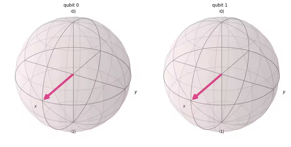
يمكننا إنشاء دائرة كمومية بكيوبتين باستخدام الكود التالي. سنُطبّق بوابة H على كل كيوبت.

# Create the two qubits quantum circuit
qc = QuantumCircuit(2)

# Apply an H gate to qubit 0
qc.h(0)

# Apply an H gate to qubit 1
qc.h(1)

# Draw the circuit
qc.draw(output="mpl")

# See the statevector
out_vector = Statevector(qc)
print(out_vector)

Statevector([0.5+0.j, 0.5+0.j, 0.5+0.j, 0.5+0.j],
            dims=(2, 2))

ملاحظة: ترتيب البتات في Qiskit

يستخدم Qiskit ترميز Little Endian عند ترتيب الكيوبتات والبتات، ما يعني أن الكيوبت 0 هو البت الموجود في أقصى اليمين في سلاسل البتات. مثال: $|01\rangle$ يعني أن q0 في الحالة $|1\rangle$ وأن q1 في الحالة $|0\rangle$. انتبه لأن بعض المراجع في الحوسبة الكمومية تستخدم ترميز Big Endian (الكيوبت 0 في أقصى اليسار)، وكذلك كثير من مراجع ميكانيكا الكم.

شيء آخر جدير بالملاحظة هو أنه عند تمثيل الدائرة الكمومية، يُوضع $|q_0\rangle$ دائمًا في أعلى الدائرة. مع أخذ هذا في الحسبان، يمكن كتابة الحالة الكمومية للدائرة أعلاه كجداء تنسوري لحالات كيوبت منفردة.

$|q1\rangle \otimes|q0\rangle = (a|0\rangle+b|1\rangle) \otimes (c|0\rangle+d|1\rangle)$

$= ac|0\rangle|0\rangle+ad|0\rangle|1\rangle+bc|1\rangle|0\rangle+bd|1\rangle|1\rangle$

$= ac|00\rangle+ad|01\rangle+bc|10\rangle+bd|11\rangle$

( $|ac|^2+ |ad|^2+ |bc|^2+ |bd|^2=1$ )

الحالة الابتدائية في Qiskit هي $|0\rangle|0\rangle=|00\rangle$، فعند تطبيق $H$ على كل كيوبت تتحول إلى حالة تراكب متساوٍ.

$H|0\rangle \otimes H|0\rangle=\frac{1}{\sqrt{2}}(|0\rangle+|1\rangle) \otimes \frac{1}{\sqrt{2}}(|0\rangle+|1\rangle) = \frac{1}{2}(|00\rangle+|01\rangle+|10\rangle+|11\rangle)$

$$=\frac{1}{2}\left( \begin{pmatrix} 1 \\ 1 \end{pmatrix} \otimes \begin{pmatrix} 1 \\ 1 \end{pmatrix}\right) = \frac{1}{2}\begin{pmatrix} 1 \\ 1 \\ 1 \\ 1 \end{pmatrix}=\frac{1}{2}\left(\begin{pmatrix} 1 \\ 0 \\ 0 \\ 0 \end{pmatrix}+\begin{pmatrix} 0 \\ 1 \\ 0 \\ 0 \end{pmatrix}+\begin{pmatrix} 0 \\ 0 \\ 1 \\ 0 \end{pmatrix}+\begin{pmatrix} 0 \\ 0 \\ 0 \\ 1 \end{pmatrix}\right)$$

قاعدة القياس هي نفسها كما في حالة الكيوبت الواحد؛ احتمالية قياس $|00\rangle$ هي $|ac|^2$.

# Draw a Bloch sphere
plot_bloch_multivector(out_vector)

الآن لنقِس هذه الدائرة.

# Create a new circuit with two qubits (first argument) and two classical bits (second argument)
qc = QuantumCircuit(2, 2)

# Apply the gates
qc.h(0)
qc.h(1)

# Add the measurement gates
qc.measure(0, 0)  # Measure qubit 0 and save the result in bit 0
qc.measure(1, 1)  # Measure qubit 1 and save the result in bit 1

# Draw the circuit
qc.draw(output="mpl")

الآن سنستخدم محاكي Aer مجددًا للتحقق تجريبيًا من أن الاحتماليات النسبية لجميع الحالات الممكنة متساوية تقريبًا.

# Run the circuit on a simulator to get the results
# Define backend
backend = AerSimulator()

# Transpile to backend
pm = generate_preset_pass_manager(backend=backend, optimization_level=1)
isa_qc = pm.run(qc)

# Run the job
sampler = Sampler(mode=backend)
job = sampler.run([isa_qc])
result = job.result()

# Print the results
counts = result[0].data.c.get_counts()
print(counts)

# Plot the counts in a histogram
plot_histogram(counts)

{'10': 262, '01': 246, '00': 265, '11': 251}

كما هو متوقع، قيست الحالات $|00\rangle$ و$|01\rangle$ و$|10\rangle$ و$|11\rangle$ بنسبة تقارب 25% لكل منها.

4.2 البوابات الكمومية متعددة الكيوبت

بوابة CNOT

بوابة CNOT (أو "NOT المتحكَّم به" أو CX) هي بوابة ثنائية الكيوبت، أي أن عملها يشمل كيوبتين في آنٍ واحد: الكيوبت المتحكِّم والكيوبت الهدف. تقلب بوابة CNOT الكيوبت الهدف فقط عندما يكون الكيوبت المتحكِّم في الحالة $|1\rangle$.

المدخل (الهدف، المتحكِّم)	المخرج (الهدف، المتحكِّم)
00	00
01	11
10	10
11	01

لنحاكِ أولًا تأثير هذه البوابة ثنائية الكيوبت عندما يكون كلٌّ من q0 وq1 في الحالة $|0\rangle$، ونستخرج متجه الحالة الناتج. الصيغة المستخدمة في Qiskit هي qc.cx(control qubit, target qubit).

# Create a circuit with two quantum registers and two classical registers
qc = QuantumCircuit(2, 2)

# Apply the CNOT (cx) gate to a |00> state.
qc.cx(0, 1)  # Here the control is set to q0 and the target is set to q1.

# Draw the circuit
qc.draw(output="mpl")

# See the statevector
out_vector = Statevector(qc)
print(out_vector)

Statevector([1.+0.j, 0.+0.j, 0.+0.j, 0.+0.j],
            dims=(2, 2))

كما هو متوقع، تطبيق بوابة CNOT على $|00\rangle$ لم يغيّر الحالة، لأن الكيوبت المتحكِّم كان في الحالة $|0\rangle$. لنعُد إلى عملية CNOT. هذه المرة سنُطبّق بوابة CNOT على $|01\rangle$ ونرى ما سيحدث.

qc = QuantumCircuit(2, 2)

# q0=1, q1=0
qc.x(0)  # Apply a X gate to initialize q0 to 1
qc.cx(0, 1)  # Set the control bit to q0 and the target bit to q1.

# Draw the circuit
qc.draw(output="mpl")

# See the statevector
out_vector = Statevector(qc)
print(out_vector)

Statevector([0.+0.j, 0.+0.j, 0.+0.j, 1.+0.j],
            dims=(2, 2))

بتطبيق بوابة CNOT، تحوّلت الحالة $|01\rangle$ إلى $|11\rangle$.

لنتحقق من هذه النتائج بتشغيل الدائرة على محاكٍ.

# Add measurements
qc.measure(0, 0)
qc.measure(1, 1)

# Draw the circuit
qc.draw(output="mpl")

# Run the circuit on a simulator to get the results
# Define backend
backend = AerSimulator()

# Transpile to backend
pm = generate_preset_pass_manager(backend=backend, optimization_level=1)
isa_qc = pm.run(qc)

# Run the job
sampler = Sampler(backend)
job = sampler.run([isa_qc])
result = job.result()

# Print the results
counts = result[0].data.c.get_counts()
print(counts)

# Plot the counts in a histogram
plot_histogram(counts)

{'11': 1024}

يُظهر الناتج أن $|11\rangle$ قيست باحتمالية 100%.

4.3 التشابك الكمومي والتنفيذ على جهاز كمومي حقيقي

لنبدأ بالتعرف على حالة متشابكة بعينها ذات أهمية خاصة في الحوسبة الكمومية، ثم سنعرّف مصطلح "التشابك":

$$\frac{1}{\sqrt{2}}|00\rangle + \frac{1}{\sqrt{2}}|11\rangle$$

وتُعرف هذه الحالة بـ حالة Bell.

الحالة المتشابكة هي حالة $|\psi_{AB}\rangle$ تتكون من حالتين كموميتين $|\psi_A\rangle$ و$|\psi_B\rangle$ لا يمكن تمثيلها كجداء تنسوري للحالات الكمومية الفردية.

إذا كانت $|\psi_{AB}\rangle$ أدناه تضم حالتين $|\psi\rangle_A$ و$|\psi\rangle_B$؛

$$|\psi_{AB}\rangle = \frac{1}{\sqrt{2}}(|00\rangle +|11\rangle) = \frac{1}{\sqrt{2}}(|0\rangle_A|0\rangle_B +|1\rangle_A|1\rangle_B)$$ $$|\psi\rangle_A = a_0|0\rangle+a_1|1\rangle$$ $$|\psi\rangle_B = b_0|0\rangle+b_1|1\rangle$$

فإن الجداء التنسوري لهاتين الحالتين هو

$$|\psi\rangle _A\otimes |\psi\rangle _B = a_0 b_0|00\rangle+a_0 b_1|01\rangle+a_1 b_0|10\rangle+a_1 b_1|11\rangle$$

لكن لا توجد معاملات $a_0, a_1, b_0,$ و$b_1$ تُحقق هاتين المعادلتين معًا. لذلك، لا يمكن تمثيل $|\psi_{AB}\rangle$ كجداء تنسوري للحالات الكمومية الفردية $|\psi\rangle_A$ و$|\psi\rangle_B$، وهذا يعني أن $|\psi_{AB}\rangle = \frac{1}{\sqrt{2}}(|00\rangle +|11\rangle)$ هي حالة متشابكة.

لنُنشئ حالة Bell ونُشغّلها على حاسوب كمومي حقيقي. سنتّبع الآن الخطوات الأربع لكتابة برنامج كمومي، المعروفة بـ أنماط Qiskit:

1. تعيين المسألة إلى دوائر ومؤثِّرات كمومية
2. التحسين لأجهزة الهدف
3. التنفيذ على جهاز الهدف
4. المعالجة اللاحقة للنتائج

الخطوة 1. تعيين المسألة إلى دوائر ومؤثِّرات كمومية

في البرنامج الكمومي، الدوائر الكمومية هي التنسيق الأصلي لتمثيل التعليمات الكمومية. عند إنشاء دائرة، ستُنشئ عادةً كائنًا جديدًا من نوع QuantumCircuit، ثم تُضيف إليه التعليمات بالتسلسل.

خلية الكود التالية تُنشئ دائرة تُولّد حالة Bell، وهي الحالة المتشابكة ثنائية الكيوبت التي ذكرناها سابقًا.

qc = QuantumCircuit(2, 2)

qc.h(0)
qc.cx(0, 1)

qc.measure(0, 0)
qc.measure(1, 1)

qc.draw("mpl")

الخطوة 2. التحسين لأجهزة الهدف

يحوّل Qiskit الدوائر المجردة إلى دوائر QISA (بنية مجموعة التعليمات الكمومية) التي تراعي قيود الجهاز الهدف وتُحسّن أداء الدائرة. لذا قبل التحسين سنُحدّد الجهاز الهدف. إن لم يكن لديك qiskit-ibm-runtime، ستحتاج إلى تثبيته أولًا. لمزيد من المعلومات حول Qiskit Runtime، راجع مرجع API.

# Install
# !pip install qiskit-ibm-runtime

سنُحدّد الجهاز الهدف.

from qiskit_ibm_runtime import QiskitRuntimeService

service = QiskitRuntimeService()
service.backends()

# You can specify the device
# backend = service.backend('ibm_kingston')

# You can also identify the least busy device
backend = service.least_busy(operational=True)
print("The least busy device is ", backend)

التحويل البرمجي للدائرة (Transpilation) هو عملية معقدة بحد ذاتها. باختصار، تُعيد كتابة الدائرة بصورة منطقية مكافئة باستخدام "البوابات الأصلية" (البوابات التي يستطيع الحاسوب الكمومي المعيّن تنفيذها)، وتربط الكيوبتات في دائرتك بالكيوبتات الحقيقية المثلى على الحاسوب الكمومي الهدف. لمزيد من التفاصيل حول التحويل البرمجي، راجع هذه الوثائق.

# Transpile the circuit into basis gates executable on the hardware
pm = generate_preset_pass_manager(backend=backend, optimization_level=1)
target_circuit = pm.run(qc)

target_circuit.draw("mpl", idle_wires=False)

يمكنك أن ترى أن الدائرة أُعيد كتابتها باستخدام بوابات جديدة خلال التحويل البرمجي. لمزيد من المعلومات، راجع توثيق ECRGate.

الخطوة 3. تنفيذ الدائرة الهدف

الآن سنُشغّل الدائرة الهدف على الجهاز الحقيقي.

sampler = Sampler(backend)
job_real = sampler.run([target_circuit])

job_id = job_real.job_id()
print("job id:", job_id)

قد يستلزم التنفيذ على الجهاز الحقيقي الانتظار في طابور، إذ تُعدّ الحواسيب الكمومية موارد ثمينة ومطلوبة بشدة. يُستخدم job_id للتحقق من حالة التنفيذ ونتائج المهمة لاحقًا.

# Check the job status (replace the job id below with your own)
job_real.status(job_id)

يمكنك أيضًا التحقق من حالة المهمة من لوحة تحكم IBM Quantum الخاصة بك: https://quantum.cloud.ibm.com/workloads

# If the Notebook session got disconnected you can also check your job status by running the following code
from qiskit_ibm_runtime import QiskitRuntimeService

service = QiskitRuntimeService()
job_real = service.job(job_id)  # Input your job-id between the quotations
job_real.status()

# Execute after job has successfully run
result_real = job_real.result()
print(result_real[0].data.c.get_counts())

الخطوة 4. المعالجة اللاحقة للنتائج

أخيرًا، يجب معالجة النتائج لإنتاج مخرجات بالتنسيق المطلوب، كالقيم أو الرسوم البيانية.

plot_histogram(result_real[0].data.c.get_counts())

كما ترى، $|00\rangle$ و$|11\rangle$ هما الأكثر ظهورًا. توجد بعض النتائج الأخرى غير المتوقعة وهي ناجمة عن الضوضاء وفقدان تماسك الكيوبت. سنتعلم المزيد عن الأخطاء والضوضاء في الحواسيب الكمومية في الدروس اللاحقة من هذه الدورة.

4.4 حالة GHZ

يمكن تمديد مفهوم التشابك إلى أنظمة تضم أكثر من كيوبتين. حالة GHZ (حالة Greenberger-Horne-Zeilinger) هي حالة متشابكة بأقصى درجة لثلاثة كيوبتات أو أكثر. تُعرَّف حالة GHZ لثلاثة كيوبتات على النحو التالي:

$$\frac{1}{\sqrt 2}(|000\rangle + |111\rangle)$$

ويمكن إنشاؤها بالدائرة الكمومية التالية.

qc = QuantumCircuit(3, 3)

qc.h(0)
qc.cx(0, 1)
qc.cx(1, 2)

qc.measure(0, 0)
qc.measure(1, 1)
qc.measure(2, 2)

qc.draw("mpl")

"العمق" (depth) هو مقياس مفيد وشائع لوصف الدوائر الكمومية. تخيّل أنك تتتبع مسارًا عبر الدائرة من اليسار إلى اليمين، مع تغيير الكيوبتات فقط عند ربطها ببوابة متعددة الكيوبتات. عدّ البوابات على طول هذا المسار؛ الحد الأقصى لعدد البوابات في أي مسار كهذا عبر الدائرة هو العمق. في الحواسيب الكمومية الحديثة المشبوبة (noisy)، الدوائر قليلة العمق تحتوي على أخطاء أقل وأرجح أن تُعطي نتائج جيدة، بينما الدوائر العميقة جدًا ليست كذلك.

باستخدام QuantumCircuit.depth()، يمكننا التحقق من عمق الدائرة الكمومية. عمق الدائرة أعلاه هو 4. أعلى كيوبت لديه ثلاث بوابات فقط بما فيها القياس، لكن يوجد مسار من الكيوبت الأعلى نزولًا إلى الكيوبت 1 أو الكيوبت 2 يتضمن بوابة CNOT إضافية.

qc.depth()

4

التمرين 2

حالة GHZ لنظام من 8 كيوبتات هي

$$\frac{1}{\sqrt 2}(|00000000\rangle + |11111111\rangle)$$

اكتب كودًا لتحضير هذه الحالة بأضحل دائرة ممكنة. عمق أضحل دائرة كمومية هو 5، بما في ذلك بوابات القياس.

الحل:

# Step 1
qc = QuantumCircuit(8, 8)

##your code goes here##
qc.h(0)
qc.cx(0, 4)
qc.cx(4, 6)
qc.cx(6, 7)

qc.cx(4, 5)

qc.cx(0, 2)
qc.cx(2, 3)

qc.cx(0, 1)
qc.barrier()  # for visual separation

# measure
for i in range(8):
    qc.measure(i, i)

qc.draw("mpl")
# print(qc.depth())

print(qc.depth())

5

from qiskit.visualization import plot_histogram
# Step 2
# For this exercise, the circuit and operators are simple, so no optimizations are needed.

# Step 3
# Run the circuit on a simulator to get the results
backend = AerSimulator()

pm = generate_preset_pass_manager(backend=backend, optimization_level=1)
isa_qc = pm.run(qc)

sampler = Sampler(mode=backend)
job = sampler.run([isa_qc], shots=1024)
result = job.result()

counts = result[0].data.c.get_counts()
print(counts)

# Step 4
# Plot the counts in a histogram

plot_histogram(counts)

{'11111111': 535, '00000000': 489}

5. الخلاصة

تعلّمت الحوسبة الكمومية بنموذج الدوائر باستخدام الكيوبتات والبوابات الكمومية، واستعرضت مفاهيم التراكب والقياس والتشابك. كما تعلّمت طريقة تنفيذ الدائرة الكمومية على جهاز كمومي حقيقي.

في التمرين الأخير لإنشاء دائرة GHZ، حاولت تقليل عمق الدائرة، وهو عامل مهم للحصول على حل ذي جدوى عملية في الحاسوب الكمومي المشبوب. في الدروس اللاحقة من هذه الدورة، ستتعلم بالتفصيل عن الضوضاء وأساليب تخفيف الأخطاء. في هذا الدرس، اعتبرنا كمقدمة تقليل عمق الدائرة في جهاز مثالي، لكن في الواقع يجب مراعاة قيود الجهاز الحقيقي كاتصالية الكيوبتات. ستتعلم المزيد عن هذا في الدروس اللاحقة من هذه الدورة.

# See the version of Qiskit
import qiskit

qiskit.__version__

'2.0.2'