المحاكاة الكمومية

ملاحظة

Yukio Kawashima (May 30, 2024)

تنزيل ملف PDF للمحاضرة الأصلية. لاحظ أن بعض مقاطع الكود قد تصبح قديمة لأنها صور ثابتة.

الوقت التقريبي للتشغيل على QPU هو 7 ثوانٍ.

(هذا الـ notebook مأخوذ في معظمه من notebook تعليمي أصبح مهجوراً الآن في Qiskit Algorithms.)

1. مقدمة

التروترة (Trotterization) هي تقنية لمحاكاة التطور الزمني الآني، وتعتمد على تطبيق متتابع لبوابات كمومية مختارة لتقريب التطور الزمني للنظام خلال شريحة زمنية صغيرة. انطلاقاً من معادلة شرودنغر، يأخذ التطور الزمني لنظام في الحالة الابتدائية $\vert\psi(0)\rangle$ الصيغة:

$$\vert \psi(t) \rangle = e^{-i H t} \vert \psi(0) \rangle \text{,}$$

حيث $H$ هو الهاميلتوني المستقل عن الزمن الذي يحكم النظام. نأخذ بعين الاعتبار هاميلتونياً يمكن كتابته على شكل مجموع موزون لحدود باولي $H=\sum_j a_j P_j$، إذ يمثل $P_j$ جداءً تنسوري لعوامل باولي تؤثر على $n$ كيوبت. قد تتبادل هذه الحدود مع بعضها أو لا تتبادل. بمعرفة الحالة عند $t=0$، كيف نحصل على حالة النظام عند وقت لاحق $|\psi(t)\rangle$ باستخدام حاسوب كمومي؟ يمكن فهم أسّي العامل بسهولة من خلال متسلسلة تايلور:

$$e^{-i H t} = 1-iHt-\frac{1}{2}H^2t^2+...$$

بعض الأسسيات البسيطة جداً، مثل $e^{iZ}$، يمكن تطبيقها بسهولة على الحواسيب الكمومية باستخدام مجموعة صغيرة من البوابات الكمومية. أما معظم الهاميلتونيات ذات الاهتمام العملي فلا تحتوي على حدٍّ واحد، بل على حدود عديدة. لاحظ ما يحدث إذا كان $H = H_1+H_2$:

$$e^{-i H t} = 1-i(H_1+H_2)t-\frac{1}{2}(H_1+H_2)^2t^2+...$$

حين يتبادل $H_1$ و$H_2$، نحصل على الحالة المألوفة (التي تنطبق أيضاً على الأعداد والمتغيرات $a$ و$b$ أدناه):

$$e^{-i (a+b) t} = e^{-i a t}e^{-i b t}$$

لكن حين لا يتبادل العاملان، لا يمكن إعادة ترتيب الحدود في متسلسلة تايلور لتبسيطها بهذه الطريقة. لذا، يُعدّ تعبير الهاميلتونيات المعقدة بشكل بوابات كمومية تحدياً قائماً.

أحد الحلول هو أخذ زمن صغير جداً $t$، بحيث يهيمن الحد الأول في توسّع تايلور. تحت هذا الافتراض:

$$e^{-i (H_1+H_2) t} \approx 1-i(H_1+H_2)t \approx (1-i H_1 t)(1-i H_2 t) \approx e^{-i H_1 t}e^{-i H_2 t}$$

بالطبع، قد نحتاج إلى تطوير حالتنا لفترة زمنية أطول. يتحقق ذلك باستخدام خطوات زمنية صغيرة متعددة. هذه العملية تُسمى التروترة:

$$\vert \psi(t) \rangle \approx \left(\prod_j e^{-i a_j P_j t/r} \right)^r \vert\psi(0) \rangle \text{,}$$

هنا $t/r$ هي الشريحة الزمنية (خطوة التطور) التي نختارها. ونتيجةً لذلك، تُنشأ بوابة تُطبَّق $r$ مرة. كلما صغرت الخطوة الزمنية، كان التقريب أدق. غير أن ذلك يُفضي إلى دوائر أعمق، مما يعني في التطبيق الفعلي تراكماً أكبر للأخطاء (وهو مصدر قلق لا يُستهان به على الأجهزة الكمومية الحديثة).

سندرس اليوم التطور الزمني لـنموذج إيزينج على شبكات خطية بحجمي $N=2$ و$N=6$ موقع. تتكون هذه الشبكات من مصفوفة من الدورانات $\sigma_i$ التي تتفاعل فقط مع جيرانها الأقرب. يمكن لهذه الدورانات أن تتخذ اتجاهين: $\uparrow$ و$\downarrow$، يقابلان مغنطة قدرها $+1$ و$-1$ على التوالي.

$$H = - J \sum_{i=0}^{N-2} Z_i Z_{i+1} - h \sum_{i=0}^{N-1} X_i \text{,}$$

حيث يصف $J$ طاقة التفاعل، و$h$ شدة المجال الخارجي (في الاتجاه x أعلاه، لكننا سنعدّل ذلك لاحقاً). لنكتب هذا التعبير باستخدام مصفوفات باولي، مع الأخذ بعين الاعتبار أن المجال الخارجي يصنع زاوية $\alpha$ مع الاتجاه المستعرض،

$$H = -J \sum_{i=0}^{N-2} Z_i Z_{i+1} -h \sum_{i=0}^{N-1} (\sin\alpha Z_i + \cos\alpha X_i) \text{.}$$

يتميز هذا الهاميلتوني بأنه يتيح لنا دراسة تأثيرات المجال الخارجي بسهولة. في الأساس الحسابي، سيُرمَّز النظام على النحو التالي:

الحالة الكمومية	تمثيل الدوران
$\lvert 0 0 0 0 \rangle$	$\uparrow\uparrow\uparrow\uparrow$
$\lvert 1 0 0 0 \rangle$	$\downarrow\uparrow\uparrow\uparrow$
$\ldots$	$\ldots$
$\lvert 1 1 1 1 \rangle$	$\downarrow\downarrow\downarrow\downarrow$

سنبدأ باستكشاف التطور الزمني لهذا النظام الكمومي، وتحديداً سنُبصِّر التطور الزمني لخصائص معينة كالمغنطة.

1.1 المتطلبات

قبل البدء بهذا الكورس، تأكد من تثبيت المكتبات التالية:

• Qiskit SDK v1.2 أو أحدث ( pip install qiskit )
• Qiskit Runtime v0.30 أو أحدث ( pip install qiskit-ibm-runtime )
• Numpy v1.24.1 أو أحدث < 2 ( pip install numpy )

1.2 استيراد المكتبات

لاحظ أن بعض المكتبات التي قد تكون مفيدة (مثل MatrixExponential وQDrift) مُدرجة حتى لو لم تُستخدم في هذا الـ notebook الحالي. يمكنك تجربتها إن كان لديك وقت!

# Added by doQumentation — required packages for this notebook
!pip install -q matplotlib numpy qiskit qiskit-ibm-runtime

# Check the version of Qiskit
import qiskit

qiskit.__version__

'2.0.2'

# Import the qiskit library
import numpy as np
import matplotlib.pylab as plt
import warnings

from qiskit import QuantumCircuit
from qiskit.circuit.library import PauliEvolutionGate
from qiskit.primitives import StatevectorEstimator
from qiskit.quantum_info import Statevector, SparsePauliOp
from qiskit.synthesis import (
    SuzukiTrotter,
    LieTrotter,
)
from qiskit.transpiler.preset_passmanagers import generate_preset_pass_manager

from qiskit_ibm_runtime import QiskitRuntimeService, SamplerV2

warnings.filterwarnings("ignore")

2. صياغة المسألة

2.1 تعريف هاميلتوني إيزينج ذي المجال المستعرض

سنأخذ هنا نموذج إيزينج أحادي البُعد ذا المجال المستعرض.

أولاً، سننشئ دالة تأخذ معاملات النظام $N$ و$J$ و$h$ و$\alpha$، وتعيد هاميلتونياتنا كـ SparsePauliOp. إن SparsePauliOp هو تمثيل متناثر لعامل كمومي بدلالة حدود Pauli الموزونة.

def get_hamiltonian(nqubits, J, h, alpha):
    # List of Hamiltonian terms as 3-tuples containing
    # (1) the Pauli string,
    # (2) the qubit indices corresponding to the Pauli string,
    # (3) the coefficient.
    ZZ_tuples = [("ZZ", [i, i + 1], -J) for i in range(0, nqubits - 1)]
    Z_tuples = [("Z", [i], -h * np.sin(alpha)) for i in range(0, nqubits)]
    X_tuples = [("X", [i], -h * np.cos(alpha)) for i in range(0, nqubits)]

    # We create the Hamiltonian as a SparsePauliOp, via the method
    # `from_sparse_list`, and multiply by the interaction term.
    hamiltonian = SparsePauliOp.from_sparse_list(
        [*ZZ_tuples, *Z_tuples, *X_tuples], num_qubits=nqubits
    )
    return hamiltonian.simplify()

تعريف الهاميلتوني

النظام الذي سندرسه الآن بحجم $N=6$، مع $J=0.2$ و$h=1.2$ و$\alpha=\frac{\pi}{8.0}$ كمثال.

n_qubits = 6

hamiltonian = get_hamiltonian(nqubits=n_qubits, J=0.2, h=1.2, alpha=np.pi / 8.0)
hamiltonian

SparsePauliOp(['IIIIZZ', 'IIIZZI', 'IIZZII', 'IZZIII', 'ZZIIII', 'IIIIIZ', 'IIIIZI', 'IIIZII', 'IIZIII', 'IZIIII', 'ZIIIII', 'IIIIIX', 'IIIIXI', 'IIIXII', 'IIXIII', 'IXIIII', 'XIIIII'],
              coeffs=[-0.2       +0.j, -0.2       +0.j, -0.2       +0.j, -0.2       +0.j,
 -0.2       +0.j, -0.45922012+0.j, -0.45922012+0.j, -0.45922012+0.j,
 -0.45922012+0.j, -0.45922012+0.j, -0.45922012+0.j, -1.10865544+0.j,
 -1.10865544+0.j, -1.10865544+0.j, -1.10865544+0.j, -1.10865544+0.j,
 -1.10865544+0.j])

2.2 ضبط معاملات محاكاة التطور الزمني

سننظر هنا في ثلاث تقنيات مختلفة للتروترة:

• Lie–Trotter (الرتبة الأولى)
• Suzuki–Trotter من الرتبة الثانية
• Suzuki–Trotter من الرتبة الرابعة

سيُستخدم الأخيران في التمرين وفي الملحق.

num_timesteps = 60
evolution_time = 30.0
dt = evolution_time / num_timesteps
product_formula_lt = LieTrotter()
product_formula_st2 = SuzukiTrotter(order=2)
product_formula_st4 = SuzukiTrotter(order=4)

2.3 إعداد الدائرة الكمومية 1 (الحالة الابتدائية)

أنشئ حالة ابتدائية. سنبدأ هنا بتهيئة دوران $\uparrow\uparrow\downarrow\downarrow\uparrow\uparrow$.

initial_circuit = QuantumCircuit(n_qubits)
initial_circuit.prepare_state("001100")
# Change reps and see the difference when you decompose the circuit
initial_circuit.decompose(reps=1).draw("mpl")

2.4 إعداد الدائرة الكمومية 2 (دائرة لخطوة زمنية واحدة)

سنبني هنا دائرة لخطوة زمنية واحدة باستخدام Lie–Trotter.

صيغة جداء لي (الرتبة الأولى) مُنفَّذة في LieTrotter. تتكون الصيغة من الدرجة الأولى من التقريب المذكور في المقدمة، حيث يُقرَّب الأسّي للمصفوفة لمجموع بجداء من الأسسيات للمصفوفات:

$$e^{H_1+H_2} \approx e^{H_1} e^{H_2}$$

كما ذكرنا سابقاً، الدوائر العميقة جداً تؤدي إلى تراكم الأخطاء وتُسبب مشكلات للحواسيب الكمومية الحديثة. نظراً لأن بوابات الكيوبتين تمتلك معدلات أخطاء أعلى من بوابات الكيوبت الواحد، فإن عمق دائرة الكيوبتين يعدّ من الأهمية بمكان. ما يهم فعلاً هو عمق دائرة الكيوبتين بعد عملية الـ transpilation (لأن ذلك هو الدائرة التي ينفذها الحاسوب الكمومي فعلاً). لكن دعنا نتعوّد على إحصاء العمليات في هذه الدائرة، حتى الآن باستخدام المحاكي.

single_step_evolution_gates_lt = PauliEvolutionGate(
    hamiltonian, dt, synthesis=product_formula_lt
)
single_step_evolution_lt = QuantumCircuit(n_qubits)
single_step_evolution_lt.append(
    single_step_evolution_gates_lt, single_step_evolution_lt.qubits
)

print(
    f"""
Trotter step with Lie-Trotter
-----------------------------
Depth: {single_step_evolution_lt.decompose(reps=3).depth()}
Gate count: {len(single_step_evolution_lt.decompose(reps=3))}
Nonlocal gate count: {single_step_evolution_lt.decompose(reps=3).num_nonlocal_gates()}
Gate breakdown: {", ".join([f"{k.upper()}: {v}" for k, v in single_step_evolution_lt.decompose(reps=3).count_ops().items()])}
"""
)
single_step_evolution_lt.decompose(reps=3).draw("mpl", fold=-1)

Trotter step with Lie-Trotter
-----------------------------
Depth: 17
Gate count: 27
Nonlocal gate count: 10
Gate breakdown: U3: 12, CX: 10, U1: 5

2.5 تحديد العوامل المراد قياسها

لنعرّف عامل المغنطة $\sum_i \langle Z_i \rangle / N$، وعامل متوسط ارتباط الدوران $\sum_i \langle Z_i Z_{i+1} \rangle/ (N - 1)$.

magnetization = (
    SparsePauliOp.from_sparse_list(
        [("Z", [i], 1.0) for i in range(0, n_qubits)], num_qubits=n_qubits
    )
    / n_qubits
)
correlation = SparsePauliOp.from_sparse_list(
    [("ZZ", [i, i + 1], 1.0) for i in range(0, n_qubits - 1)], num_qubits=n_qubits
) / (n_qubits - 1)
print("magnetization : ", magnetization)
print("correlation : ", correlation)

magnetization :  SparsePauliOp(['IIIIIZ', 'IIIIZI', 'IIIZII', 'IIZIII', 'IZIIII', 'ZIIIII'],
              coeffs=[0.16666667+0.j, 0.16666667+0.j, 0.16666667+0.j, 0.16666667+0.j,
 0.16666667+0.j, 0.16666667+0.j])
correlation :  SparsePauliOp(['IIIIZZ', 'IIIZZI', 'IIZZII', 'IZZIII', 'ZZIIII'],
              coeffs=[0.2+0.j, 0.2+0.j, 0.2+0.j, 0.2+0.j, 0.2+0.j])

2.6 تنفيذ محاكاة التطور الزمني

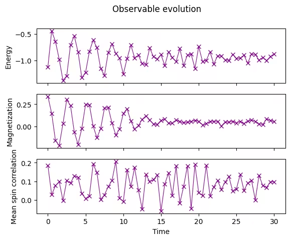
سنتابع الطاقة (القيمة المتوقعة للهاميلتوني)، والمغنطة (القيمة المتوقعة لعامل المغنطة)، ومتوسط ارتباط الدوران (القيمة المتوقعة لعامل الارتباط). يُقدّر StatevectorEstimator (EstimatorV2) في Qiskit القيم المتوقعة للمراقبات، $\langle\psi\vert\hat{O}\vert\psi\rangle$.

# Initiate the circuit
evolved_state = QuantumCircuit(initial_circuit.num_qubits)
# Start from the initial spin configuration
evolved_state.append(initial_circuit, evolved_state.qubits)
# Initiate Estimator (V2)
estimator = StatevectorEstimator()
# Set number of shots
shots = 10000
# Translate the precision required from the number of shots
precision = np.sqrt(1 / shots)
energy_list = []
mag_list = []
corr_list = []
# Estimate expectation values for t=0.0
job = estimator.run(
    [(evolved_state, [hamiltonian, magnetization, correlation])], precision=precision
)
# Get estimated expectation values
evs = job.result()[0].data.evs
energy_list.append(evs[0])
mag_list.append(evs[1])
corr_list.append(evs[2])
# Start time evolution
for n in range(num_timesteps):
    # Expand the circuit to describe delta-t
    evolved_state.append(single_step_evolution_gates_lt, evolved_state.qubits)
    # Estimate expectation values at delta-t
    job = estimator.run(
        [(evolved_state, [hamiltonian, magnetization, correlation])],
        precision=precision,
    )
    # Retrieve results (expectation values)
    evs = job.result()[0].data.evs
    energy_list.append(evs[0])
    mag_list.append(evs[1])
    corr_list.append(evs[2])
# Transform the list of expectation values (at each time step) to arrays
energy_array = np.array(energy_list)
mag_array = np.array(mag_list)
corr_array = np.array(corr_list)

2.7 رسم التطور الزمني للمراقبات

سنرسم القيم المتوقعة التي قسناها مقابل الزمن.

fig, axes = plt.subplots(3, sharex=True)
times = np.linspace(0, evolution_time, num_timesteps + 1)  # includes initial state
axes[0].plot(
    times,
    energy_array,
    label="First order",
    marker="x",
    c="darkmagenta",
    ls="-",
    lw=0.8,
)
axes[1].plot(
    times, mag_array, label="First order", marker="x", c="darkmagenta", ls="-", lw=0.8
)
axes[2].plot(
    times, corr_array, label="First order", marker="x", c="darkmagenta", ls="-", lw=0.8
)
axes[0].set_ylabel("Energy")
axes[1].set_ylabel("Magnetization")
axes[2].set_ylabel("Mean spin correlation")
axes[2].set_xlabel("Time")
fig.suptitle("Observable evolution")

Text(0.5, 0.98, 'Observable evolution')

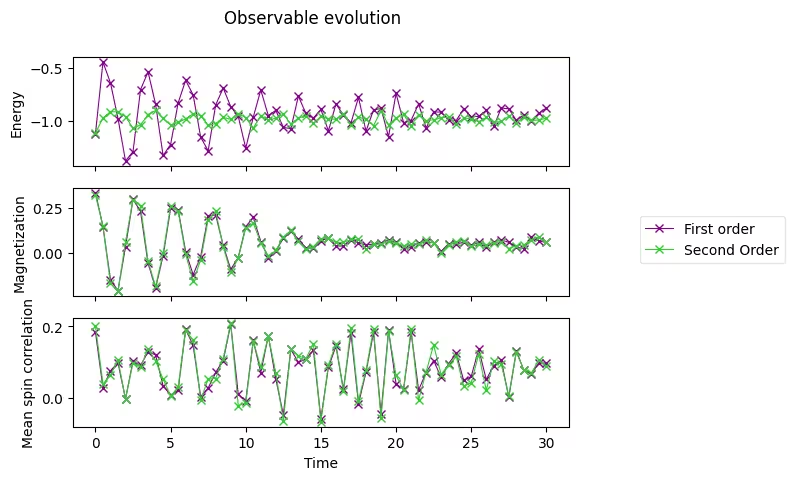
3. التمرين الأول: تنفيذ المحاكاة باستخدام Suzuki–Trotter من الرتبة الثانية

لنجرب الآن تنفيذ المحاكاة باستخدام Suzuki–Trotter من الرتبة الثانية، على غرار مثال Lie–Trotter الموضّح أعلاه.

يمكن استخدام Suzuki–Trotter من الرتبة الثانية في Qiskit عبر SuzukiTrotter class. باستخدام هذه الصيغة، يكون التحليل من الدرجة الثانية:

$$e^{H_1+H_2} \approx e^{H_1/2}e^{H_2}e^{H_1/2}$$

3.1 بناء دائرة لخطوة زمنية واحدة

استخدم product_formula_st2 (SuzukiTrotter(order=2)) وابنِ دائرة لخطوة زمنية واحدة باستخدام Suzuki–Trotter من الرتبة الثانية. احسب أيضاً عدد البوابات وعمق الدائرة وقارنها مع Lie–Trotter.

# Modify the line below (Use PauliEvolutionGate)
single_step_evolution_gates_st2 = PauliEvolutionGate(
    hamiltonian, dt, synthesis=product_formula_st2
)
single_step_evolution_st2 = QuantumCircuit(n_qubits)
single_step_evolution_st2.append(
    single_step_evolution_gates_st2, single_step_evolution_st2.qubits
)
# Let us print some stats
print(
    f"""
Trotter step with second-order Suzuki-Trotter
-----------------------------
Depth: {single_step_evolution_st2.decompose(reps=3).depth()}
Gate count: {len(single_step_evolution_st2.decompose(reps=3))}
Nonlocal gate count: {single_step_evolution_st2.decompose(reps=3).num_nonlocal_gates()}
Gate breakdown: {", ".join([f"{k.upper()}: {v}" for k, v in single_step_evolution_st2.decompose(reps=3).count_ops().items()])}
"""
)
single_step_evolution_st2.decompose(reps=2).draw("mpl", fold=-1)

Trotter step with second-order Suzuki-Trotter
-----------------------------
Depth: 34
Gate count: 53
Nonlocal gate count: 20
Gate breakdown: U3: 23, CX: 20, U1: 10

3.2 تنفيذ محاكاة التطور الزمني

نفّذ التطور الزمني باستخدام Suzuki–Trotter من الرتبة الثانية.

# Initiate the circuit
evolved_state = QuantumCircuit(initial_circuit.num_qubits)
# Start from the initial spin configuration
evolved_state.append(initial_circuit, evolved_state.qubits)
# Initiate Estimator (V2)
estimator = StatevectorEstimator()
# Set number of shots
shots = 10000
# Translate the precision required from the number of shots
precision = np.sqrt(1 / shots)
energy_list_st2 = []
mag_list_st2 = []
corr_list_st2 = []
# Estimate expectation values for t=0.0
job = estimator.run(
    [(evolved_state, [hamiltonian, magnetization, correlation])], precision=precision
)
# Get estimated expectation values
evs = job.result()[0].data.evs
energy_list_st2.append(evs[0])
mag_list_st2.append(evs[1])
corr_list_st2.append(evs[2])
# Start time evolution
for n in range(num_timesteps):
    # Expand the circuit to describe delta-t
    evolved_state.append(single_step_evolution_gates_st2, evolved_state.qubits)
    # Estimate expectation values at delta-t
    job = estimator.run(
        [(evolved_state, [hamiltonian, magnetization, correlation])],
        precision=precision,
    )
    # Retrieve results (expectation values)
    evs = job.result()[0].data.evs
    energy_list_st2.append(evs[0])
    mag_list_st2.append(evs[1])
    corr_list_st2.append(evs[2])
# Transform the list of expectation values (at each time step) to arrays
energy_array_st2 = np.array(energy_list_st2)
mag_array_st2 = np.array(mag_list_st2)
corr_array_st2 = np.array(corr_list_st2)

3.3 رسم نتائج Suzuki–Trotter من الرتبة الثانية

axes[0].plot(
    times,
    energy_array_st2,
    label="Second Order",
    marker="x",
    c="limegreen",
    ls="-",
    lw=0.8,
)
axes[1].plot(
    times,
    mag_array_st2,
    label="Second Order",
    marker="x",
    c="limegreen",
    ls="-",
    lw=0.8,
)
axes[2].plot(
    times,
    corr_array_st2,
    label="Second Order",
    marker="x",
    c="limegreen",
    ls="-",
    lw=0.8,
)

# Replace the legend
# legend.remove()
legend = fig.legend(
    *axes[0].get_legend_handles_labels(),
    bbox_to_anchor=(1.0, 0.5),
    loc="center left",
    framealpha=0.5,
)
fig

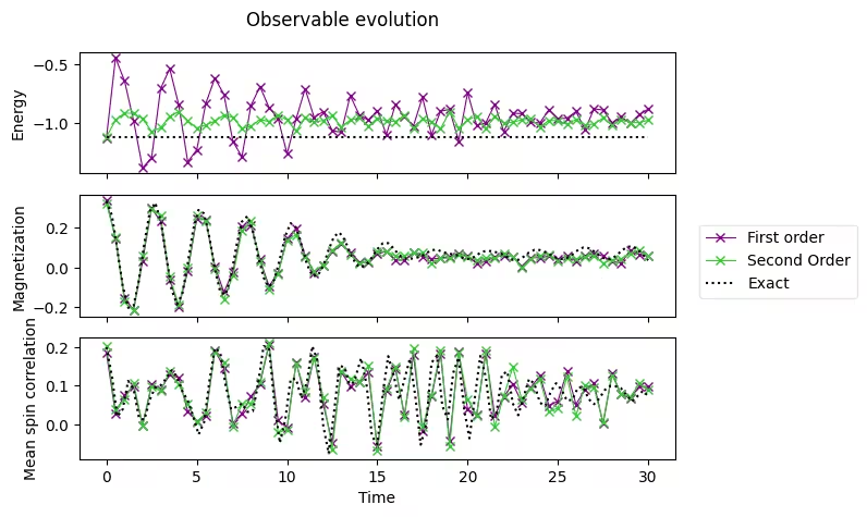
3.4 المقارنة مع النتائج الدقيقة

البيانات التالية هي النتائج الدقيقة المحسوبة مسبقاً بالحاسوب الكلاسيكي.

exact_times = np.array(
    [
        0.0,
        0.3,
        0.6,
        0.8999999999999999,
        1.2,
        1.5,
        1.7999999999999998,
        2.1,
        2.4,
        2.6999999999999997,
        3.0,
        3.3,
        3.5999999999999996,
        3.9,
        4.2,
        4.5,
        4.8,
        5.1,
        5.3999999999999995,
        5.7,
        6.0,
        6.3,
        6.6,
        6.8999999999999995,
        7.199999999999999,
        7.5,
        7.8,
        8.1,
        8.4,
        8.7,
        9.0,
        9.299999999999999,
        9.6,
        9.9,
        10.2,
        10.5,
        10.799999999999999,
        11.1,
        11.4,
        11.7,
        12.0,
        12.299999999999999,
        12.6,
        12.9,
        13.2,
        13.5,
        13.799999999999999,
        14.1,
        14.399999999999999,
        14.7,
        15.0,
        15.299999999999999,
        15.6,
        15.899999999999999,
        16.2,
        16.5,
        16.8,
        17.099999999999998,
        17.4,
        17.7,
        18.0,
        18.3,
        18.599999999999998,
        18.9,
        19.2,
        19.5,
        19.8,
        20.099999999999998,
        20.4,
        20.7,
        21.0,
        21.3,
        21.599999999999998,
        21.9,
        22.2,
        22.5,
        22.8,
        23.099999999999998,
        23.4,
        23.7,
        24.0,
        24.3,
        24.599999999999998,
        24.9,
        25.2,
        25.5,
        25.8,
        26.099999999999998,
        26.4,
        26.7,
        27.0,
        27.3,
        27.599999999999998,
        27.9,
        28.2,
        28.5,
        28.799999999999997,
        29.099999999999998,
        29.4,
        29.7,
        30.0,
    ]
)
exact_energy = np.array(
    [
        -1.1184402376762155,
        -1.1184402376762157,
        -1.1184402376762157,
        -1.1184402376762148,
        -1.1184402376762153,
        -1.1184402376762155,
        -1.1184402376762148,
        -1.118440237676216,
        -1.118440237676216,
        -1.1184402376762166,
        -1.1184402376762148,
        -1.118440237676216,
        -1.1184402376762153,
        -1.1184402376762148,
        -1.118440237676217,
        -1.118440237676215,
        -1.1184402376762161,
        -1.1184402376762157,
        -1.118440237676217,
        -1.1184402376762161,
        -1.1184402376762137,
        -1.1184402376762161,
        -1.1184402376762161,
        -1.118440237676218,
        -1.1184402376762155,
        -1.1184402376762166,
        -1.1184402376762155,
        -1.1184402376762137,
        -1.1184402376762186,
        -1.1184402376762215,
        -1.1184402376762148,
        -1.118440237676216,
        -1.1184402376762166,
        -1.1184402376762148,
        -1.1184402376762121,
        -1.1184402376762166,
        -1.1184402376762181,
        -1.1184402376762137,
        -1.1184402376762148,
        -1.1184402376762193,
        -1.1184402376762108,
        -1.1184402376762144,
        -1.118440237676217,
        -1.1184402376762197,
        -1.1184402376762153,
        -1.1184402376762161,
        -1.1184402376762184,
        -1.1184402376762126,
        -1.118440237676214,
        -1.118440237676214,
        -1.1184402376762161,
        -1.118440237676212,
        -1.1184402376762164,
        -1.118440237676217,
        -1.1184402376762121,
        -1.1184402376762157,
        -1.1184402376762212,
        -1.1184402376762217,
        -1.1184402376762206,
        -1.118440237676222,
        -1.1184402376762166,
        -1.118440237676212,
        -1.1184402376762137,
        -1.11844023767622,
        -1.1184402376762206,
        -1.118440237676219,
        -1.1184402376762153,
        -1.1184402376762164,
        -1.118440237676209,
        -1.1184402376762144,
        -1.1184402376762161,
        -1.118440237676216,
        -1.1184402376762173,
        -1.118440237676214,
        -1.1184402376762093,
        -1.1184402376762184,
        -1.1184402376762126,
        -1.118440237676213,
        -1.1184402376762195,
        -1.1184402376762095,
        -1.1184402376762075,
        -1.1184402376762197,
        -1.1184402376762141,
        -1.1184402376762146,
        -1.1184402376762184,
        -1.118440237676218,
        -1.1184402376762224,
        -1.118440237676219,
        -1.118440237676218,
        -1.1184402376762206,
        -1.1184402376762168,
        -1.118440237676221,
        -1.118440237676218,
        -1.1184402376762148,
        -1.1184402376762106,
        -1.1184402376762173,
        -1.118440237676216,
        -1.118440237676216,
        -1.1184402376762113,
        -1.1184402376762275,
        -1.1184402376762195,
    ]
)
exact_magnetization = np.array(
    [
        0.3333333333333333,
        0.26316769633415005,
        0.0912947227110664,
        -0.09317712543141576,
        -0.20391854332115245,
        -0.19318196655046493,
        -0.06411527074401464,
        0.12558269854206197,
        0.28252754464640606,
        0.3264196194042506,
        0.2361586169847769,
        0.060894367906122224,
        -0.10842387093076275,
        -0.18636359582538073,
        -0.1338364343947887,
        0.020284606520827753,
        0.19151142743926025,
        0.2905341647678381,
        0.2723014646745304,
        0.15147481733047252,
        -0.008179102877790292,
        -0.1242999208732406,
        -0.1372529247781061,
        -0.04083616185958952,
        0.11066094926716476,
        0.23140661570567636,
        0.2587109403786205,
        0.1868237670027325,
        0.061201779383143744,
        -0.051391248969654205,
        -0.09843899603365061,
        -0.061297056158849166,
        0.04199010081939773,
        0.15861461430963147,
        0.22336830674799552,
        0.20179555623336537,
        0.11407111438609417,
        0.01609419104778282,
        -0.04239611796730001,
        -0.04249123521065924,
        0.008850291714888112,
        0.08780898151558082,
        0.1561486776507056,
        0.17627348772811832,
        0.13870676179652253,
        0.07205869195282538,
        0.018300003064909465,
        0.0001095640839572417,
        0.015157929316037586,
        0.05077755280969454,
        0.09245534457650838,
        0.12206907551110702,
        0.12284950557969157,
        0.09570215398601932,
        0.06294378255078983,
        0.045503313813986014,
        0.043389819499542556,
        0.046725117769796744,
        0.054956411358382404,
        0.0713814528253614,
        0.08743689703248492,
        0.08951216359166674,
        0.07878386475305985,
        0.06955669116405788,
        0.06639892435963689,
        0.05890378761746903,
        0.04541796525844558,
        0.0414221088331947,
        0.05499634106912299,
        0.07409418836014572,
        0.08371859070160165,
        0.08211623987959302,
        0.07615055161378328,
        0.06702584458783024,
        0.051891407742740085,
        0.038049378383635625,
        0.03825614149768043,
        0.054183218463525695,
        0.0753534475741016,
        0.08853147112587295,
        0.08767917178542013,
        0.07709383184439536,
        0.06308595032042386,
        0.0498812359204284,
        0.04299040064096167,
        0.04769159891460652,
        0.06483569572288776,
        0.08698035745435016,
        0.10047391641776235,
        0.09747255683203637,
        0.08098863187287358,
        0.05959496723987331,
        0.04383882265040485,
        0.04232138798062125,
        0.05720514169944535,
        0.08201306299870219,
        0.10274898262000469,
        0.10707552455080133,
        0.09210856128265357,
        0.06379922105742579,
        0.03624325103307953,
    ]
)
exact_correlation = np.array(
    [
        0.2,
        0.1247704225763532,
        0.01943938494098705,
        0.03854917181332821,
        0.11196616231067426,
        0.0906546700356683,
        0.01629373561896267,
        0.011352652889791095,
        0.0636185676540077,
        0.09543834437789013,
        0.10058518161011307,
        0.11829217731417431,
        0.1397812224038133,
        0.12316460402216707,
        0.08541383059335775,
        0.06144846844403662,
        0.020246372880505827,
        -0.02693683090021662,
        0.003919250903281282,
        0.1117419430168554,
        0.19676155181256794,
        0.18594408880783336,
        0.1002673802566004,
        0.03821525827438024,
        0.04485205090247377,
        0.05348102743040269,
        0.03160026140008638,
        0.033437649060464834,
        0.10486939975320728,
        0.20249469538955758,
        0.19735507621013149,
        0.0553097261765083,
        -0.04889114490131667,
        0.011685690974970964,
        0.11705971535823065,
        0.11681165998194759,
        0.06637091239560744,
        0.10936684225958895,
        0.20225454101061405,
        0.16284420833341812,
        -0.0025823294931362067,
        -0.0763416631752919,
        0.02985268630418397,
        0.15234468006771007,
        0.14606385406970995,
        0.0935341856492092,
        0.12325421854361143,
        0.17130422930386324,
        0.10383730044042278,
        -0.031333159406547614,
        -0.05241572078596815,
        0.07722509925347705,
        0.17642188574256007,
        0.12765340239966838,
        0.06309968945093776,
        0.11574687130499339,
        0.16978282647206913,
        0.0736143632571229,
        -0.05356602733119409,
        -0.0009649396796768892,
        0.15921620111869142,
        0.17760366431811037,
        0.04736297330213485,
        0.012122870263181897,
        0.13268065586830521,
        0.1728473023503636,
        0.03999259331072221,
        -0.036997053070222885,
        0.06951528580242439,
        0.1769169993516561,
        0.12290448295710298,
        0.012897784654866427,
        0.02859435620982225,
        0.12895847695150875,
        0.13629536955485938,
        0.05394621059822597,
        0.02298040588184324,
        0.07036499900317271,
        0.11706448623132719,
        0.10435285842074606,
        0.055721236329964965,
        0.04676334743672697,
        0.08417924910022263,
        0.10611161955304965,
        0.089304171047322,
        0.06098589533081194,
        0.06314519797488709,
        0.09431492621892917,
        0.09667836915967139,
        0.0651298357290882,
        0.05176966009147416,
        0.06727229484222669,
        0.08871788283607947,
        0.09907054249093444,
        0.09785167773502176,
        0.09277216140054353,
        0.07520999642062785,
        0.05894392248382922,
        0.07236135251622376,
        0.08608284185200156,
        0.07282922961856123,
    ]
)

axes[0].plot(exact_times, exact_energy, c="k", ls=":", label="Exact")
axes[1].plot(exact_times, exact_magnetization, c="k", ls=":", label="Exact")
axes[2].plot(exact_times, exact_correlation, c="k", ls=":", label="Exact")
# Replace the legend
legend.remove()
# Select the labels of only the first axis
legend = fig.legend(
    *axes[0].get_legend_handles_labels(),
    bbox_to_anchor=(1.0, 0.5),
    loc="center left",
    framealpha=0.5,
)
fig.tight_layout()
fig

4. التنفيذ على العتاد الكمي

بعد ذلك، سنشغّل محاكاة التطور الزمني على العتاد الكمي الفعلي. سنعمل على مسألة أصغر بحجم شبكة N=2، ونغيّر قيمة المعامل $\alpha$ لنرى الفرق في ديناميكية دالة الموجة.

4.1 الخطوة 1. تحويل المدخلات الكلاسيكية إلى مسألة كمية

اختر الإعدادات الأولية للمحاكاة:

n_qubits_2 = 2
dt_2 = 1.6
product_formula = LieTrotter(reps=1)

ثم عيّن الدائرة الابتدائية:

التهيئة الأولية للأسبين ستكون "أسفل-أعلى"

# We prepare an initial state ↓↑ (10).
# Note that Statevector and SparsePauliOp interpret the qubits from right to left
initial_circuit_2 = QuantumCircuit(n_qubits_2)
initial_circuit_2.prepare_state("10")
# Change reps and see the difference when you decompose the circuit
initial_circuit_2.decompose(reps=1).draw("mpl")

احسب الآن القيمة المرجعية باستخدام محاكي statevector مثالي.

bar_width = 0.1
# initial_state = Statevector.from_label("10")
final_time = 1.6
eps = 1e-5

# We create the list of angles in radians, with a small epsilon
# the exactly longitudinal field, which would present no dynamics at all
alphas = np.linspace(-np.pi / 2 + eps, np.pi / 2 - eps, 5)

for i, alpha in enumerate(alphas):
    evolved_state_2 = QuantumCircuit(initial_circuit_2.num_qubits)
    evolved_state_2.append(initial_circuit_2, evolved_state_2.qubits)
    hamiltonian_2 = get_hamiltonian(nqubits=2, J=0.2, h=1.0, alpha=alpha)
    single_step_evolution_gates_2 = PauliEvolutionGate(
        hamiltonian_2, dt_2, synthesis=product_formula
    )
    evolved_state_2.append(single_step_evolution_gates_2, evolved_state_2.qubits)
    evolved_state_2 = Statevector(evolved_state_2)
    # Dictionary of probabilities
    amplitudes_dict = evolved_state_2.probabilities_dict()
    labels = list(amplitudes_dict.keys())
    values = list(amplitudes_dict.values())
    # Convert angle to degrees
    alpha_str = f"$\\alpha={int(np.round(alpha * 180 / np.pi))}^\\circ$"
    plt.bar(np.arange(4) + i * bar_width, values, bar_width, label=alpha_str, alpha=0.7)

plt.xticks(np.arange(4) + 2 * bar_width, labels)
plt.xlabel("Measurement")
plt.ylabel("Probability")
plt.suptitle(
    f"Measurement probabilities at $t={final_time}$, for various field angles $\\alpha$\n"
    f"Initial state: 10, Linear lattice of size $L=2$"
)
plt.legend()

<matplotlib.legend.Legend at 0x11c816590>

قمنا بتهيئة النظام بتسلسل أسبينات $\downarrow\uparrow$، وهو ما يقابل $\vert\psi(0)\rangle = \vert10\rangle$. بعد تركه يتطور لزمن $t=1.6$ تحت تأثير حقل عرضي ($\alpha=0^\circ$)، يكاد يكون من المؤكد أننا سنقيس $\uparrow\downarrow$، أي حدوث تبادل للأسبين. (لاحظ أن التسميات تُقرأ من اليمين إلى اليسار). أما إذا كان الحقل طوليًا ($\alpha=\pm90^\circ$)، فلن يحدث أي تطور، وسنقيس النظام كما هيّأناه في البداية $\downarrow\uparrow$. وعند الزوايا المتوسطة $\alpha=\pm45^\circ$، ستظهر كل التوليفات الممكنة باحتمالات مختلفة، وسيكون تبادل الأسبين الأكثر احتمالًا بنسبة 67%.

بناء الدائرة لتجربة العتاد الكمي

circuit_list = []
for i, alpha in enumerate(alphas):
    evolved_state_2 = QuantumCircuit(initial_circuit_2.num_qubits)
    evolved_state_2.append(initial_circuit_2, evolved_state_2.qubits)
    hamiltonian_2 = get_hamiltonian(nqubits=2, J=0.2, h=1.0, alpha=alpha)
    single_step_evolution_gates_2 = PauliEvolutionGate(
        hamiltonian_2, dt_2, synthesis=product_formula
    )
    evolved_state_2.append(single_step_evolution_gates_2, evolved_state_2.qubits)
    evolved_state_2.measure_all()
    circuit_list.append(evolved_state_2)

4.2 الخطوة 2. التحسين لاستهداف العتاد المطلوب

نحدد الـ Backend المستهدف.

service = QiskitRuntimeService()
backend = service.least_busy(operational=True, simulator=False)
backend.name

'ibm_strasbourg'

بعد ذلك، نجري عملية Transpile للدائرة ليتناسب مع الـ Backend المختار.

pm = generate_preset_pass_manager(backend=backend, optimization_level=3)
circuit_isa = pm.run(circuit_list)

تحقق من الدائرة.

circuit_isa[1].draw("mpl", idle_wires=False)

4.3 الخطوة 3. التنفيذ باستخدام Qiskit Runtime primitives

توفر أداة Sampler (الإصدار V2) في Qiskit عدد bitstrings المقاسة.

sampler = SamplerV2(mode=backend)
job = sampler.run(circuit_isa)
job_id = job.job_id()
print("job id:", job_id)

job id: d13pswfmya70008ek070

احفظ النتائج

results = job.result()

4.4 الخطوة 4. معالجة النتائج

ابنِ مخطط الرسم البياني لـ bitstrings، وهو ما يعادل تحليل دالة الموجة، وقارنها بالقيم المثالية المعروضة أعلاه.

list_temp = ["00", "01", "10", "11"]

for i, alpha in enumerate(alphas):
    # Dictionary of probabilities
    amplitudes_dict = results[i].data.meas.get_counts()
    values = []
    for str_temp in list_temp:
        values.append(
            amplitudes_dict[str_temp] / 4096.0
        )  # divided by default number of shots
    # Convert angle to degrees
    alpha_str = f"$\\alpha={int(np.round(alpha * 180 / np.pi))}^\\circ$"
    plt.bar(np.arange(4) + i * bar_width, values, bar_width, label=alpha_str, alpha=0.7)

plt.xticks(np.arange(4) + 2 * bar_width, labels)
plt.xlabel("Measurement")
plt.ylabel("Probabilities")
plt.suptitle(
    f"Measurement probabilities at $t={final_time}$, for various field angles $\\alpha$\n"
    f"Initial state: 10, Linear lattice of size $L=2$"
)
plt.legend()

<matplotlib.legend.Legend at 0x11d7af990>

نعرض هنا مثالًا على بناء دائرة باستخدام صيغة Suzuki–Trotter من الرتبة الرابعة. دعنا الآن نجرّب بناء محاكاة دائرة باستخدام Suzuki–Trotter من الرتبة الرابعة تبعًا للأمثلة الموضحة أعلاه.

يمكن استخدام Suzuki–Trotter من الرتبة الرابعة في Qiskit عبر فئة SuzukiTrotter. يمكن حساب الرتبة الرابعة باستخدام علاقة التكرار التالية. لاحظ أن رتبة Suzuki–Trotter تُشار إليها بـ "2k" في المعادلات التالية.

$$\hat{U}_{ST(2k)}\left(t\right) = \left[ \hat{U}_{ST(2k-2)}\left(p_k t\right) \right]^2 \hat{U}_{ST(2k-2)}\left( (1- 4 p_k) t\right)\left[ \hat{U}_{ST(2k-2)}\left(p_k t\right) \right]^2$$ $$p_k = 1 / \left(4-4^{\frac{1}{2k-1}}\right)$$

بناء دائرة لخطوة زمنية واحدة

استخدم product_formula_st4 (SuzukiTrotter(order=4)) وابنِ دائرة لخطوة زمنية واحدة باستخدام Suzuki–Trotter من الرتبة الرابعة. أيضًا، احسب عدد البوابات وعمق الدائرة وقارنهما مع Lie–Trotter و Suzuki–Trotter من الرتبة الثانية.

# Modify the line below (Use PauliEvolutionGate)
single_step_evolution_gates_st4 = PauliEvolutionGate(
    hamiltonian, dt, synthesis=product_formula_st4
)
single_step_evolution_st4 = QuantumCircuit(n_qubits)
single_step_evolution_st4.append(
    single_step_evolution_gates_st4, single_step_evolution_st4.qubits
)
# Let us print some stats
print(
    f"""
Trotter step with second-order Suzuki-Trotter
-----------------------------
Depth: {single_step_evolution_st4.decompose(reps=3).depth()}
Gate count: {len(single_step_evolution_st4.decompose(reps=3))}
Nonlocal gate count: {single_step_evolution_st4.decompose(reps=3).num_nonlocal_gates()}
Gate breakdown: {", ".join([f"{k.upper()}: {v}" for k, v in single_step_evolution_st4.decompose(reps=3).count_ops().items()])}
"""
)
single_step_evolution_st4.decompose(reps=2).draw("mpl", fold=-1)

Trotter step with second-order Suzuki-Trotter
-----------------------------
Depth: 170
Gate count: 265
Nonlocal gate count: 100
Gate breakdown: U3: 115, CX: 100, U1: 50

# Check Qiskit version
import qiskit

qiskit.__version__

'2.0.2'