محاكاة هاميلتوني إيزنج المُركَل باستخدام الدوائر الديناميكية

تقدير الاستخدام: 7.5 دقيقة على معالج Heron r3. (ملاحظة: هذا تقدير فحسب. قد يختلف وقت التشغيل الفعلي.) الدوائر الديناميكية هي دوائر تتضمن تغذية أمامية كلاسيكية - أي أنها قياسات تُجرى في منتصف الدائرة تعقبها عمليات منطق كلاسيكية تحدد العمليات الكمومية المشروطة بالناتج الكلاسيكي. في هذا الدرس، نحاكي نموذج إيزنج المُركَل على شبكة سداسية من الدورانات، ونستخدم الدوائر الديناميكية لتحقيق تفاعلات تتجاوز الاتصال الفيزيائي للعتاد.

لقد خُضِع نموذج إيزنج لدراسة مستفيضة في مختلف مجالات الفيزياء. يُنمذج هذا النظامُ دوراناتٍ تخضع لتفاعلات إيزنج بين مواقع الشبكة، فضلاً عن ركلات من المجال المغناطيسي المحلي في كل موقع. يُعطى التطور الزمني لـ Trotter للدورانات المدروس في هذا الدرس، المأخوذ من [1]، بالوحدوي التالي:

$$U(\theta)=\left(\prod_{\langle j, k\rangle} \exp \left(i \frac{\pi}{8} Z_j Z_k\right)\right)\left(\prod_j \exp \left(-i \frac{\theta}{2} X_j\right)\right)$$

لاستقصاء ديناميكيات الدوران، ندرس متوسط مغنطة الدورانات في كل موقع دالةً في خطوات Trotter. ومن ثَمَّ نبني الرصيد القابل للرصد التالي:

$$\langle O\rangle = \frac{1}{N} \sum_i \langle Z_i \rangle$$

لتحقيق تفاعل ZZ بين مواقع الشبكة، نعرض حلاً يعتمد على ميزة الدائرة الديناميكية، مما يُفضي إلى عمق ثنائي الكيوبت أقصر بكثير مقارنةً بأسلوب التوجيه القياسي باستخدام بوابات SWAP. في المقابل، تستغرق عمليات التغذية الأمامية الكلاسيكية في الدوائر الديناميكية وقتاً أطول عادةً من البوابات الكمومية؛ لذا تنطوي الدوائر الديناميكية على قيود ومفاضلات. كما نعرض طريقةً لإضافة تسلسل عزل ديناميكي على الكيوبتات الخاملة خلال عملية التغذية الأمامية الكلاسيكية باستخدام مدة stretch.

المتطلبات

قبل البدء بهذا الدرس، تأكد من تثبيت ما يلي:

• Qiskit SDK الإصدار 2.0 أو أحدث مع دعم التصور المرئي
• Qiskit Runtime الإصدار 0.37 أو أحدث مع دعم التصور المرئي (pip install 'qiskit-ibm-runtime[visualization]')
• مكتبة الرسم البياني Rustworkx (pip install rustworkx)
• Qiskit Aer (pip install qiskit-aer)

الإعداد

import numpy as np
from typing import List
import rustworkx as rx
import matplotlib.pyplot as plt
from rustworkx.visualization import mpl_draw
from qiskit.circuit import (
    Parameter,
    QuantumCircuit,
    QuantumRegister,
    ClassicalRegister,
)
from qiskit.transpiler import CouplingMap
from qiskit.quantum_info import SparsePauliOp
from qiskit.circuit.classical import expr
from qiskit.transpiler.preset_passmanagers import (
    generate_preset_pass_manager,
)
from qiskit.transpiler import PassManager
from qiskit.circuit.library import RZGate, XGate
from qiskit.transpiler.passes import (
    ALAPScheduleAnalysis,
    PadDynamicalDecoupling,
)

from qiskit.transpiler.basepasses import TransformationPass
from qiskit.circuit.measure import Measure
from qiskit.transpiler.passes.utils.remove_final_measurements import (
    calc_final_ops,
)
from qiskit.circuit import Instruction

from qiskit.visualization import plot_circuit_layout
from qiskit.circuit.tools import pi_check

from qiskit_aer import AerSimulator
from qiskit_aer.primitives import SamplerV2 as Aer_Sampler

from qiskit_ibm_runtime import (
    QiskitRuntimeService,
    Batch,
    SamplerV2 as Sampler,
)
from qiskit_ibm_runtime.exceptions import QiskitBackendNotFoundError
from qiskit_ibm_runtime.visualization import (
    draw_circuit_schedule_timing,
)

الخطوة 1: تعيين المدخلات الكلاسيكية إلى دائرة كمومية

نبدأ بتعريف الشبكة المراد محاكاتها. نختار العمل مع الشبكة السداسية (المعروفة أيضاً بشبكة خلية النحل)، وهي رسم بياني مستوٍ بعُقد من الدرجة 3. هنا نحدد حجم الشبكة، ومعاملات الدائرة ذات الصلة في ديناميكيات Trotter. نحاكي التطور الزمني لـ Trotter تحت نموذج إيزنج بثلاث قيم مختلفة لـ $\theta$ للمجال المغناطيسي المحلي.

hex_rows = 3  # specify lattice size
hex_cols = 5
depths = range(9)  # specify Trotter steps
zz_angle = np.pi / 8  # parameter for ZZ interaction
max_angle = np.pi / 2  # max theta angle
points = 3  # number of theta parameters

θ = Parameter("θ")
params = np.linspace(0, max_angle, points)

def make_hex_lattice(hex_rows=1, hex_cols=1):
    """Define hexagon lattice."""
    hex_cmap = CouplingMap.from_hexagonal_lattice(
        hex_rows, hex_cols, bidirectional=False
    )
    data = list(hex_cmap.physical_qubits)
    graph = hex_cmap.graph.to_undirected(multigraph=False)
    edge_colors = rx.graph_misra_gries_edge_color(graph)
    layer_edges = {color: [] for color in edge_colors.values()}
    for edge_index, color in edge_colors.items():
        layer_edges[color].append(graph.edge_list()[edge_index])
    return data, layer_edges, hex_cmap, graph

لنبدأ بمثال اختبار صغير:

hex_rows_test = 1
hex_cols_test = 2

data_test, layer_edges_test, hex_cmap_test, graph_test = make_hex_lattice(
    hex_rows=hex_rows_test, hex_cols=hex_cols_test
)

# display a small example for illustration
node_colors_test = ["lightblue"] * len(graph_test.node_indices())
pos = rx.graph_spring_layout(
    graph_test,
    k=5 / np.sqrt(len(graph_test.nodes())),
    repulsive_exponent=1,
    num_iter=150,
)
mpl_draw(graph_test, node_color=node_colors_test, pos=pos)

سنستخدم المثال الصغير للتوضيح والمحاكاة. فيما يلي، نبني أيضاً مثالاً كبيراً لإظهار إمكانية توسيع سير العمل إلى أحجام أكبر.

data, layer_edges, hex_cmap, graph = make_hex_lattice(
    hex_rows=hex_rows, hex_cols=hex_cols
)
num_qubits = len(data)
print(f"num_qubits = {num_qubits}")

# display the honeycomb lattice to simulate
node_colors = ["lightblue"] * len(graph.node_indices())
pos = rx.graph_spring_layout(
    graph,
    k=5 / np.sqrt(num_qubits),
    repulsive_exponent=1,
    num_iter=150,
)
mpl_draw(graph, node_color=node_colors, pos=pos)
plt.show()

num_qubits = 46

بناء الدوائر الوحدوية

مع تحديد حجم المسألة والمعاملات، نحن الآن مستعدون لبناء الدائرة ذات المعاملات التي تحاكي التطور الزمني لـ Trotter لـ $U(\theta)$ بخطوات Trotter مختلفة، المحددة بالوسيط depth. تتضمن الدائرة التي نبنيها طبقات متناوبة من بوابات Rx($\theta$) وبوابات Rzz. تُحقق بوابات Rzz تفاعلات ZZ بين الدورانات المقترنة، وستُوضع بين كل موقع من مواقع الشبكة المحددة بالوسيط layer_edges.

def gen_hex_unitary(
    num_qubits=6,
    zz_angle=np.pi / 8,
    layer_edges=[
        [(0, 1), (2, 3), (4, 5)],
        [(1, 2), (3, 4), (5, 0)],
    ],
    θ=Parameter("θ"),
    depth=1,
    measure=False,
    final_rot=True,
):
    """Build unitary circuit."""
    circuit = QuantumCircuit(num_qubits)
    # Build trotter layers
    for _ in range(depth):
        for i in range(num_qubits):
            circuit.rx(θ, i)
        circuit.barrier()
        for coloring in layer_edges.keys():
            for e in layer_edges[coloring]:
                circuit.rzz(zz_angle, e[0], e[1])
        circuit.barrier()
    # Optional final rotation, set True to be consistent with Ref. [1]
    if final_rot:
        for i in range(num_qubits):
            circuit.rx(θ, i)
    if measure:
        circuit.measure_all()

    return circuit

تصور دائرة الاختبار الصغيرة:

circ_unitary_test = gen_hex_unitary(
    num_qubits=len(data_test),
    layer_edges=layer_edges_test,
    θ=Parameter("θ"),
    depth=1,
    measure=True,
)
circ_unitary_test.draw(output="mpl", fold=-1)

وبالمثل، ابنِ الدوائر الوحدوية للمثال الكبير عند خطوات Trotter المختلفة، والرصيد القابل للرصد لتقدير قيمة التوقع.

circuits_unitary = []
for depth in depths:
    circ = gen_hex_unitary(
        num_qubits=num_qubits,
        layer_edges=layer_edges,
        θ=Parameter("θ"),
        depth=depth,
        measure=True,
    )
    circuits_unitary.append(circ)

observables_unitary = SparsePauliOp.from_sparse_list(
    [("Z", [i], 1 / num_qubits) for i in range(num_qubits)],
    num_qubits=num_qubits,
)

بناء تطبيق الدائرة الديناميكية

يوضح هذا القسم التطبيق الرئيسي للدائرة الديناميكية لمحاكاة التطور الزمني ذاته لـ Trotter. لاحظ أن شبكة خلية النحل التي نريد محاكاتها لا تتطابق مع الشبكة الثقيلة لكيوبتات العتاد. إحدى الطرق المباشرة لتعيين الدائرة على العتاد هي إدخال سلسلة من عمليات SWAP لإحضار الكيوبتات المتفاعلة بجانب بعضها لتحقيق تفاعل ZZ. هنا نسلط الضوء على نهج بديل باستخدام الدوائر الديناميكية كحل، مما يوضح أنه بإمكاننا استخدام توليفة من الحسابين الكمومي والكلاسيكي في الوقت الحقيقي داخل دائرة في Qiskit لتحقيق تفاعلات تتجاوز أقرب الجيران.

في تطبيق الدائرة الديناميكية، يُنفَّذ تفاعل ZZ فعلياً باستخدام كيوبتات مساعدة وقياسات في منتصف الدائرة وتغذية أمامية. لفهم ذلك، لاحظ أن دورات ZZ تُطبق عاملاً طوري $e^{i\theta}$ على الحالة بناءً على تكافؤها. بالنسبة لكيوبتين، حالات الأساس الحسابي هي $|00\rangle$، و$|01\rangle$، و$|10\rangle$، و$|11\rangle$. تُطبق بوابة دوران ZZ عاملاً طورياً على الحالتين $|01\rangle$ و$|10\rangle$ اللتين تكافؤهما (عدد الوحدات في الحالة) فردي، وتترك الحالات ذات التكافؤ الزوجي دون تغيير. يصف ما يلي كيف يمكننا تطبيق تفاعلات ZZ على كيوبتين بفاعلية باستخدام الدوائر الديناميكية.

1. حساب التكافؤ في كيوبت مساعد: بدلاً من تطبيق ZZ مباشرةً على كيوبتين، نُدخل كيوبتاً ثالثاً، هو الكيوبت المساعد، لتخزين معلومات التكافؤ للكيوبتين الخاصَّين بالبيانات. نشابك الكيوبت المساعد مع كل كيوبت بيانات باستخدام بوابات CX من كيوبت البيانات إلى الكيوبت المساعد.

2. تطبيق دوران Z أحادي الكيوبت على الكيوبت المساعد: ذلك لأن الكيوبت المساعد يحتوي على معلومات التكافؤ للكيوبتين الخاصَّين بالبيانات، مما يُنفذ دوران ZZ على كيوبتَي البيانات بصورة فعلية.

3. قياس الكيوبت المساعد في أساس X: هذه هي الخطوة المحورية التي تُؤدي إلى انهيار حالة الكيوبت المساعد، ونتيجة القياس تخبرنا بما حدث:

   • قياس 0: عند رصد نتيجة 0، نكون قد طبقنا دوران $ZZ(\theta)$ بصورة صحيحة على كيوبتَي البيانات.

   • قياس 1: عند رصد نتيجة 1، نكون قد طبقنا $ZZ(\theta + \pi)$ عوضاً عن ذلك.

4. تطبيق بوابة تصحيح عند قياس 1: إذا قسنا القيمة 1، نُطبق بوابات Z على كيوبتَي البيانات لـ"إصلاح" الطور الزائد $\pi$.

الدائرة الناتجة هي التالية:

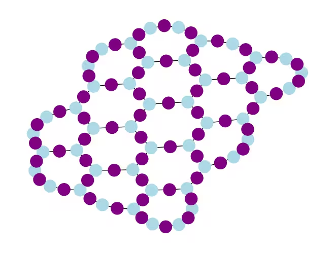
عند اعتماد هذا النهج لمحاكاة شبكة خلية النحل، تنتظم الدائرة الناتجة بشكل مثالي في العتاد ذي الشبكة السداسية الثقيلة: تقع جميع كيوبتات البيانات على مواقع الشبكة ذات الدرجة 3، التي تشكل شبكة سداسية. يتشارك كل زوج من كيوبتات البيانات في كيوبت مساعد يقع على موقع من الدرجة 2. فيما يلي، نبني شبكة الكيوبتات لتطبيق الدائرة الديناميكية، مُدخِلين كيوبتات مساعدة (موضحة بالدوائر البنفسجية الداكنة).

def make_lattice(hex_rows=1, hex_cols=1):
    """Define heavy-hex lattice and corresponding lists of data and ancilla nodes."""
    hex_cmap = CouplingMap.from_hexagonal_lattice(
        hex_rows, hex_cols, bidirectional=False
    )
    data = list(hex_cmap.physical_qubits)

    heavyhex_cmap = CouplingMap()
    for d in data:
        heavyhex_cmap.add_physical_qubit(d)

    # make coupling map
    a = len(data)
    for edge in hex_cmap.get_edges():
        heavyhex_cmap.add_physical_qubit(a)
        heavyhex_cmap.add_edge(edge[0], a)
        heavyhex_cmap.add_edge(edge[1], a)
        a += 1
    ancilla = list(range(len(data), a))
    qubits = data + ancilla

    # color edges
    graph = heavyhex_cmap.graph.to_undirected(multigraph=False)
    edge_colors = rx.graph_misra_gries_edge_color(graph)
    layer_edges = {color: [] for color in edge_colors.values()}
    for edge_index, color in edge_colors.items():
        layer_edges[color].append(graph.edge_list()[edge_index])

    # construct observable
    obs_hex = SparsePauliOp.from_sparse_list(
        [("Z", [i], 1 / len(data)) for i in data],
        num_qubits=len(qubits),
    )

    return (data, qubits, ancilla, layer_edges, heavyhex_cmap, graph, obs_hex)

تصور شبكة heavy-hex لكيوبتات البيانات والكيوبتات المساعدة على نطاق صغير:

(data, qubits, ancilla, layer_edges, heavyhex_cmap, graph, obs_hex) = (
    make_lattice(hex_rows=hex_rows, hex_cols=hex_cols)
)

print(f"number of data qubits = {len(data)}")
print(f"number of ancilla qubits = {len(ancilla)}")

node_colors = []
for node in graph.node_indices():
    if node in ancilla:
        node_colors.append("purple")
    else:
        node_colors.append("lightblue")

pos = rx.graph_spring_layout(
    graph,
    k=1 / np.sqrt(len(qubits)),
    repulsive_exponent=2,
    num_iter=200,
)

# Visualize the graph, blue circles are data qubits and purple circles are ancillas
mpl_draw(graph, node_color=node_colors, pos=pos)
plt.show()

number of data qubits = 46
number of ancilla qubits = 60

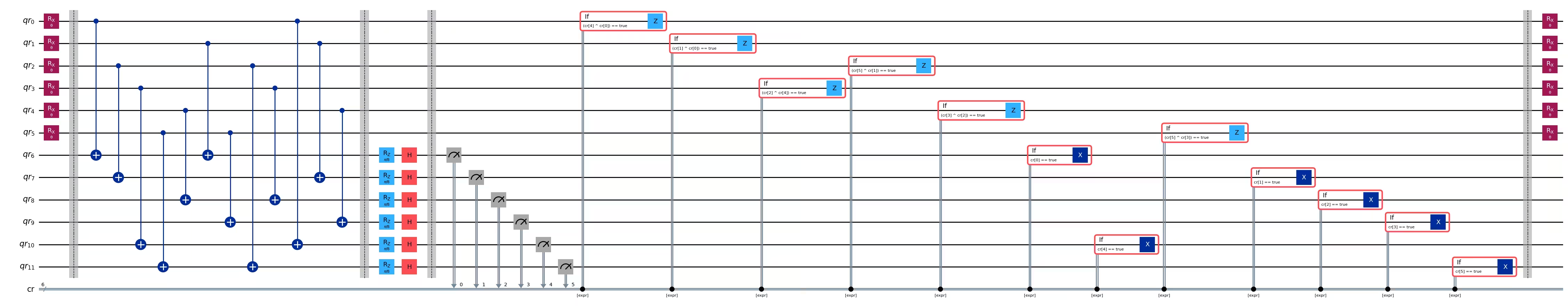
فيما يلي، نبني الدائرة الديناميكية للتطور الزمني لـ Trotter. تُستبدل بوابات RZZ بتطبيق الدائرة الديناميكية باتباع الخطوات الموصوفة أعلاه.

def gen_hex_dynamic(
    depth=1,
    zz_angle=np.pi / 8,
    θ=Parameter("θ"),
    hex_rows=1,
    hex_cols=1,
    measure=False,
    add_dd=True,
):
    """Build dynamic circuits."""
    (data, qubits, ancilla, layer_edges, heavyhex_cmap, graph, obs_hex) = (
        make_lattice(hex_rows=hex_rows, hex_cols=hex_cols)
    )
    # Initialize circuit
    qr = QuantumRegister(len(qubits), "qr")
    cr = ClassicalRegister(len(ancilla), "cr")
    circuit = QuantumCircuit(qr, cr)

    for k in range(depth):
        # Single-qubit Rx layer
        for d in data:
            circuit.rx(θ, d)
        circuit.barrier()

        # CX gates from data qubits to ancilla qubits
        for same_color_edges in layer_edges.values():
            for e in same_color_edges:
                circuit.cx(e[0], e[1])
        circuit.barrier()

        # Apply Rz rotation on ancilla qubits and rotate into X basis
        for a in ancilla:
            circuit.rz(zz_angle, a)
            circuit.h(a)
        # Add barrier to align terminal measurement
        circuit.barrier()

        # Measure ancilla qubits
        for i, a in enumerate(ancilla):
            circuit.measure(a, i)
        d2ros = {}
        a2ro = {}
        # Retrieve ancilla measurement outcomes
        for a in ancilla:
            a2ro[a] = cr[ancilla.index(a)]

        # For each data qubit, retrieve measurement outcomes of neighboring ancilla qubits
        for d in data:
            ros = [a2ro[a] for a in heavyhex_cmap.neighbors(d)]
            d2ros[d] = ros

        # Build classical feedforward operations (optionally add DD on idling data qubits)
        for d in data:
            if add_dd:
                circuit = add_stretch_dd(circuit, d, f"data_{d}_depth_{k}")

            # # XOR the neighboring readouts of the data qubit; if True, apply Z to it
            ros = d2ros[d]
            parity = ros[0]
            for ro in ros[1:]:

            for ro in ros[1:]:
                parity = expr.bit_xor(parity, ro)
            with circuit.if_test(expr.equal(parity, True)):
                circuit.z(d)

        # Reset the ancilla if its readout is 1
        for a in ancilla:
            with circuit.if_test(expr.equal(a2ro[a], True)):
                circuit.x(a)
        circuit.barrier()

    # Final single-qubit Rx layer to match the unitary circuits
    for d in data:
        circuit.rx(θ, d)

    if measure:
        circuit.measure_all()
    return circuit, obs_hex

def add_stretch_dd(qc, q, name):
    """Add XpXm DD sequence."""
    s = qc.add_stretch(name)
    qc.delay(s, q)
    qc.x(q)
    qc.delay(s, q)
    qc.delay(s, q)
    qc.rz(np.pi, q)
    qc.x(q)
    qc.rz(-np.pi, q)
    qc.delay(s, q)
    return qc

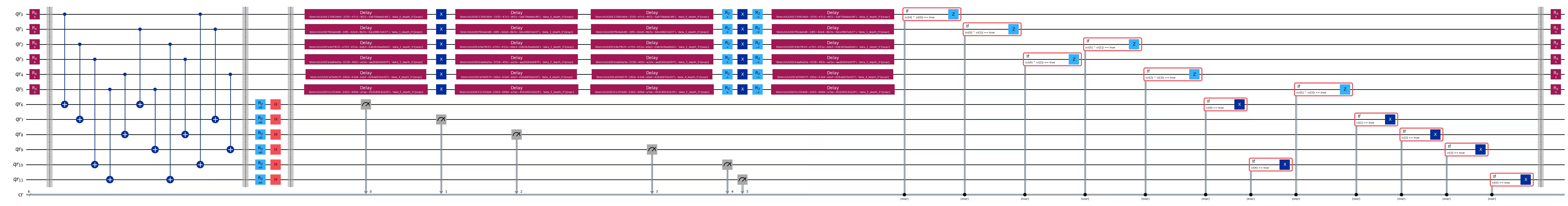
الفصل الديناميكي (DD) ودعم مدة stretch

أحد التحفظات في استخدام تنفيذ الدوائر الديناميكية لتحقيق تفاعل ZZ هو أن قياس الدائرة أثناء التشغيل وعمليات التغذية الراجعة الكلاسيكية تستغرق عادةً وقتاً أطول في التنفيذ مقارنةً بالبوابات الكمومية. لقمع تفكك الكيوبت أثناء وقت الخمول الناتج عن العمليات الكلاسيكية، أضفنا تسلسل الفصل الديناميكي (DD) بعد عملية القياس على كيوبتات ancilla، وقبل عملية Z المشروطة على كيوبت البيانات، أي قبل عبارة if_test.

يُضاف تسلسل DD عبر الدالة add_stretch_dd()، التي تستخدم مدد stretch لتحديد الفترات الزمنية بين بوابات DD. مدة stretch هي طريقة لتحديد مدة زمنية قابلة للتمدد لعملية delay، بحيث يمكن أن تنمو مدة التأخير لملء وقت خمول الكيوبت. يتم حل متغيرات المدة المحددة بواسطة stretch في وقت الترجمة إلى مدد مطلوبة تفي بقيود معينة. وهذا مفيد للغاية عندما يكون توقيت تسلسلات DD ضرورياً لتحقيق أداء جيد في قمع الأخطاء. لمزيد من التفاصيل حول نوع stretch، راجع توثيق OpenQASM. حالياً، دعم نوع stretch في Qiskit Runtime تجريبي. للاطلاع على تفاصيل قيود استخدامه، يرجى الرجوع إلى قسم القيود في توثيق stretch.

باستخدام الدوال المحددة أعلاه، نبني دوائر التطور الزمني بأسلوب Trotter، مع DD وبدونه، والمقاسات المقابلة لها. نبدأ بتصور الدائرة الديناميكية لمثال صغير:

hex_rows_test = 1
hex_cols_test = 1

(
    data_test,
    qubits_test,
    ancilla_test,
    layer_edges_test,
    heavyhex_cmap_test,
    graph_test,
    obs_hex_test,
) = make_lattice(hex_rows=hex_rows_test, hex_cols=hex_cols_test)

node_colors = []
for node in graph_test.node_indices():
    if node in ancilla_test:
        node_colors.append("purple")
    else:
        node_colors.append("lightblue")
pos = rx.graph_spring_layout(
    graph_test,
    k=5 / np.sqrt(len(qubits_test)),
    repulsive_exponent=2,
    num_iter=150,
)

# display a small example for illustration
node_colors_test = ["lightblue"] * len(graph_test.node_indices())
mpl_draw(graph_test, node_color=node_colors, pos=pos)

circuit_dynamic_test, obs_dynamic_test = gen_hex_dynamic(
    depth=1,
    θ=Parameter("θ"),
    hex_rows=hex_rows_test,
    hex_cols=hex_cols_test,
    measure=False,
    add_dd=False,
)
circuit_dynamic_test.draw("mpl", fold=-1)

circuit_dynamic_dd_test, _ = gen_hex_dynamic(
    depth=1,
    θ=Parameter("θ"),
    hex_rows=hex_rows_test,
    hex_cols=hex_cols_test,
    measure=False,
    add_dd=True,
)
circuit_dynamic_dd_test.draw("mpl", fold=-1)

وبالمثل، نبني الدوائر الديناميكية للمثال الكبير:

circuits_dynamic = []
circuits_dynamic_dd = []
observables_dynamic = []
for depth in depths:
    circuit, obs = gen_hex_dynamic(
        depth=depth,
        θ=Parameter("θ"),
        hex_rows=hex_rows,
        hex_cols=hex_cols,
        measure=True,
        add_dd=False,
    )
    circuits_dynamic.append(circuit)

    circuit_dd, _ = gen_hex_dynamic(
        depth=depth,
        θ=Parameter("θ"),
        hex_rows=hex_rows,
        hex_cols=hex_cols,
        measure=True,
        add_dd=True,
    )
    circuits_dynamic_dd.append(circuit_dd)
    observables_dynamic.append(obs)

الخطوة 2: تحسين المسألة لتنفيذها على العتاد

أصبحنا الآن جاهزين لترجمة الدائرة إلى العتاد. سنترجم كلاً من التنفيذ الموحد القياسي وتنفيذ الدائرة الديناميكية إلى العتاد.

لتحويل الدائرة إلى العتاد، نبدأ أولاً بإنشاء مثيل للخلفية (backend). إذا كان متاحاً، سنختار خلفية تدعم تعليمة MidCircuitMeasure (أي measure_2).

service = QiskitRuntimeService()
try:
    backend = service.least_busy(
        operational=True,
        simulator=False,
        use_fractional_gates=True,
        filters=lambda b: "measure_2" in b.supported_instructions,
    )
except QiskitBackendNotFoundError:
    backend = service.least_busy(
        operational=True,
        simulator=False,
        use_fractional_gates=True,
    )

الترجمة للدوائر الديناميكية

أولاً، نترجم الدوائر الديناميكية مع إضافة تسلسل DD وبدونه. لضمان استخدام نفس مجموعة الكيوبتات الفيزيائية في جميع الدوائر للحصول على نتائج أكثر اتساقاً، نترجم الدائرة مرة واحدة أولاً، ثم نستخدم تخطيطها لجميع الدوائر اللاحقة، المحدد بواسطة initial_layout في pass manager. ثم نبني كتل موحدة أساسية (PUBs) كمدخلات لأداة Sampler.

pm_temp = generate_preset_pass_manager(
    optimization_level=3,
    backend=backend,
)
isa_temp = pm_temp.run(circuits_dynamic[-1])
dynamic_layout = isa_temp.layout.initial_index_layout(filter_ancillas=True)

pm = generate_preset_pass_manager(
    optimization_level=3, backend=backend, initial_layout=dynamic_layout
)

dynamic_isa_circuits = [pm.run(circ) for circ in circuits_dynamic]
dynamic_pubs = [(circ, params) for circ in dynamic_isa_circuits]

dynamic_isa_circuits_dd = [pm.run(circ) for circ in circuits_dynamic_dd]
dynamic_pubs_dd = [(circ, params) for circ in dynamic_isa_circuits_dd]

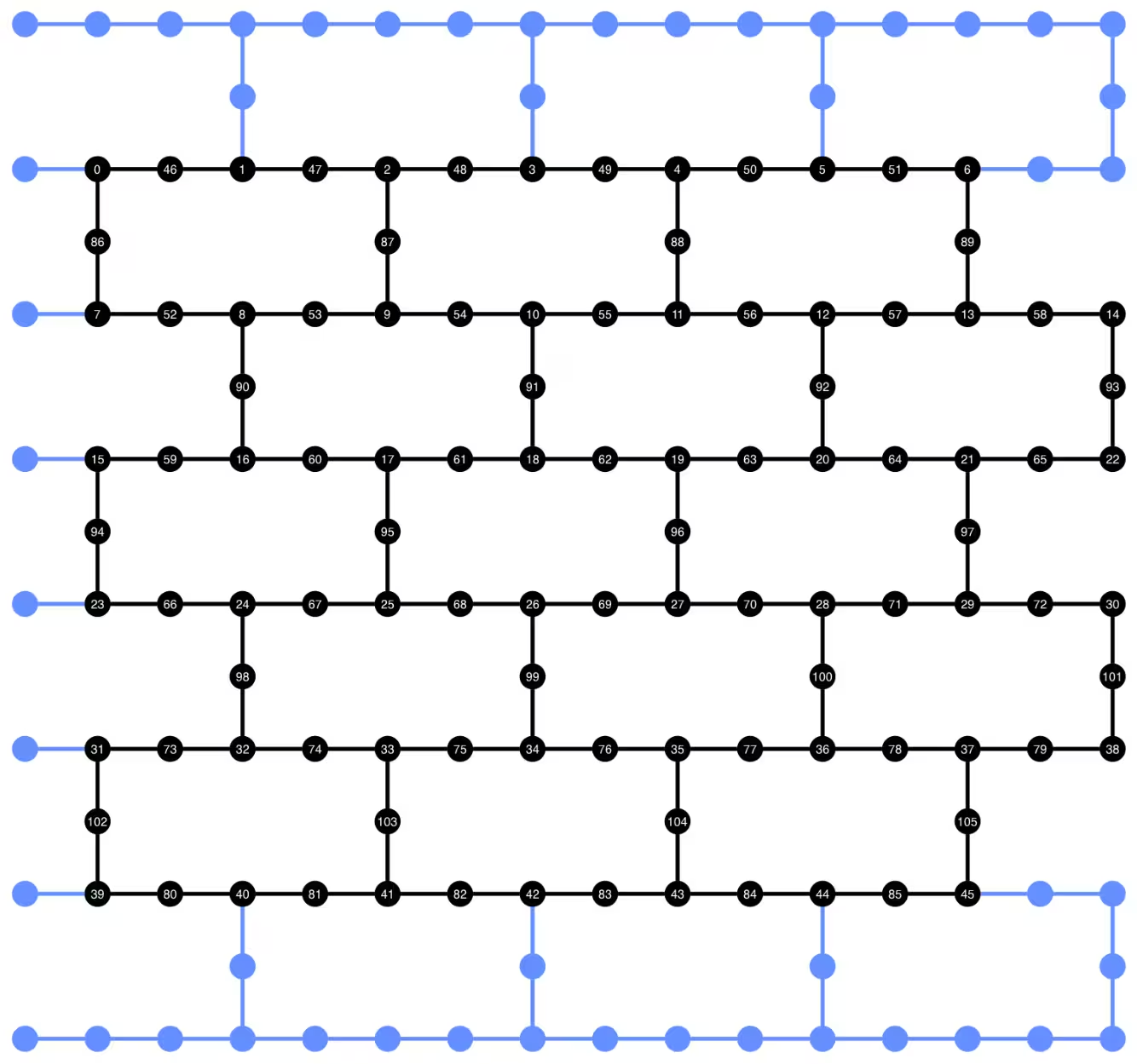
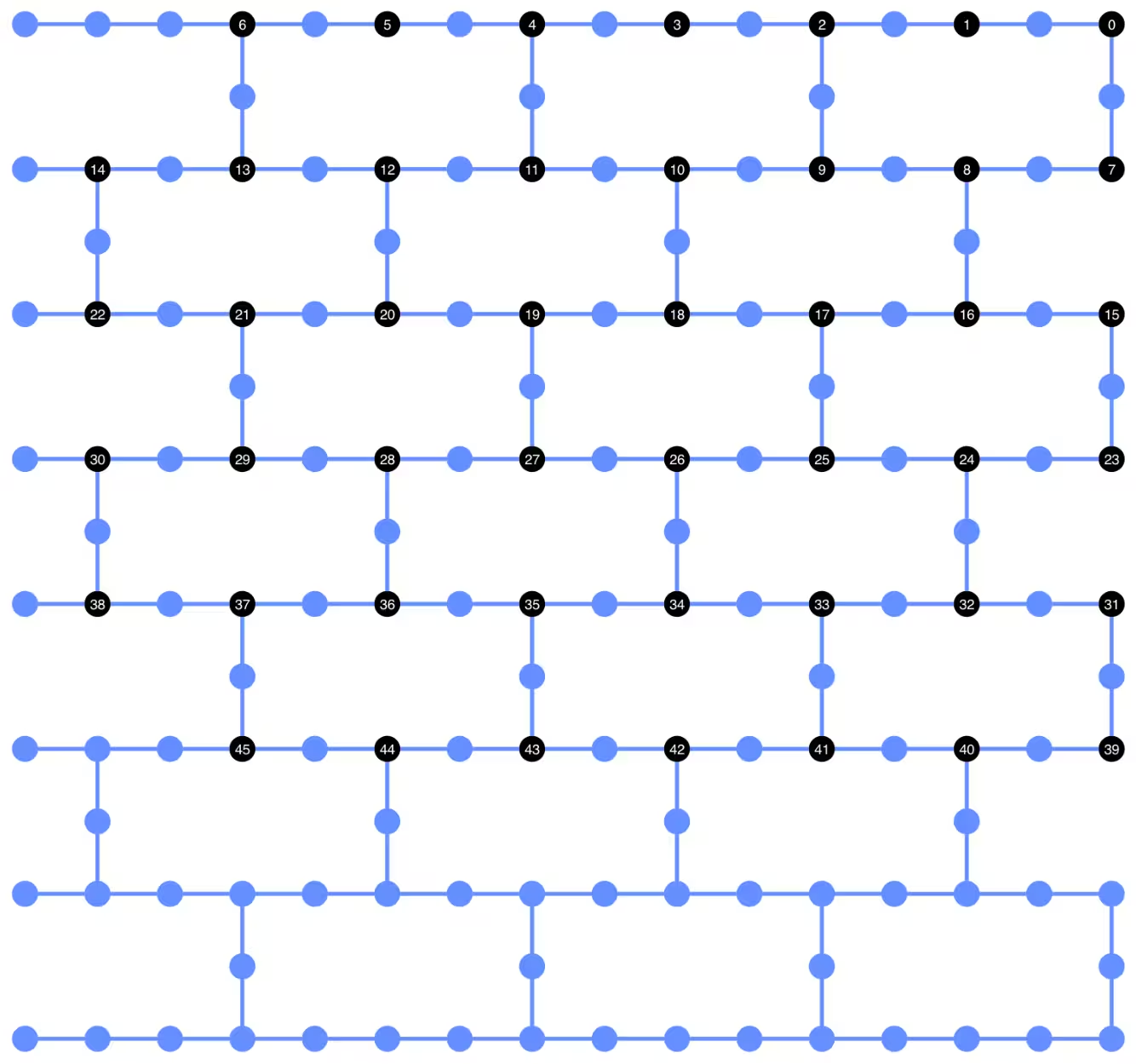
يمكننا تصور تخطيط الكيوبت للدائرة المترجمة أدناه. تُظهر الدوائر السوداء كيوبتات البيانات وكيوبتات ancilla المستخدمة في تنفيذ الدائرة الديناميكية.

def _heron_coords_r2():
    cord_map = np.array(
        [
            [
                0,
                1,
                2,
                3,
                4,
                5,
                6,
                7,
                8,
                9,
                10,
                11,
                12,
                13,
                14,
                15,
                3,
                7,
                11,
                15,
                0,
                1,
                2,
                3,
                4,
                5,
                6,
                7,
                8,
                9,
                10,
                11,
                12,
                13,
                14,
                15,
                1,
                5,
                9,
                13,
                0,
                1,
                2,
                3,
                4,
                5,
                6,
                7,
                8,
                9,
                10,
                11,
                12,
                13,
                14,
                15,
                3,
                7,
                11,
                15,
                0,
                1,
                2,
                3,
                4,
                5,
                6,
                7,
                8,
                9,
                10,
                11,
                12,
                13,
                14,
                15,
                1,
                5,
                9,
                13,
                0,
                1,
                2,
                3,
                4,
                5,
                6,
                7,
                8,
                9,
                10,
                11,
                12,
                13,
                14,
                15,
                3,
                7,
                11,
                15,
                0,
                1,
                2,
                3,
                4,
                5,
                6,
                7,
                8,
                9,
                10,
                11,
                12,
                13,
                14,
                15,
                1,
                5,
                9,
                13,
                0,
                1,
                2,
                3,
                4,
                5,
                6,
                7,
                8,
                9,
                10,
                11,
                12,
                13,
                14,
                15,
                3,
                7,
                11,
                15,
                0,
                1,
                2,
                3,
                4,
                5,
                6,
                7,
                8,
                9,
                10,
                11,
                12,
                13,
                14,
                15,
            ],
            -1
            * np.array([j for i in range(15) for j in [i] * [16, 4][i % 2]]),
        ],
        dtype=int,
    )

    hcords = []
    ycords = cord_map[0]
    xcords = cord_map[1]
    for i in range(156):
        hcords.append([xcords[i] + 1, np.abs(ycords[i]) + 1])

    return hcords

plot_circuit_layout(
    dynamic_isa_circuits_dd[8],
    backend,
    qubit_coordinates=_heron_coords_r2(),
    view="virtual",
)

ملاحظة

إذا واجهت أخطاء تفيد بعدم العثور على neato من plot_circuit_layout()، فتأكد من تثبيت حزمة graphviz وإتاحتها في متغير PATH لديك. إذا تم تثبيتها في موقع غير افتراضي (على سبيل المثال، باستخدام homebrew على MacOS)، فقد تحتاج إلى تحديث متغير بيئة PATH. يمكن إجراء ذلك داخل هذا الدفتر باستخدام ما يلي:

import os
os.environ['PATH'] = f"path/to/neato{os.pathsep}{os.environ['PATH']}"

dynamic_isa_circuits[1].draw(fold=-1, output="mpl", idle_wires=False)

dynamic_isa_circuits_dd[1].draw(fold=-1, output="mpl", idle_wires=False)

الترجمة باستخدام MidCircuitMeasure

MidCircuitMeasure هو إضافة إلى عمليات القياس المتاحة، مُعايَر خصيصاً لإجراء قياسات الدائرة أثناء التشغيل. تُعيَّن تعليمة MidCircuitMeasure إلى تعليمة measure_2 التي تدعمها الخلفيات. لاحظ أن measure_2 غير مدعوم على جميع الخلفيات. يمكنك استخدام service.backends(filters=lambda b: "measure_2" in b.supported_instructions) للعثور على الخلفيات التي تدعمه. هنا، نوضح كيفية ترجمة الدائرة بحيث يتم تنفيذ قياسات الدائرة أثناء التشغيل المحددة في الدائرة باستخدام عملية MidCircuitMeasure، إذا كانت الخلفية تدعمها.

أدناه، نطبع المدة الزمنية لتعليمة measure_2 والتعليمة القياسية measure.

print(
    f'Mid-circuit measurement `measure_2` duration: {backend.instruction_durations.get('measure_2',0) * backend.dt * 1e9/1e3} μs'
)
print(
    f'Terminal measurement `measure` duration: {backend.instruction_durations.get('measure',0) * backend.dt *1e9/1e3} μs'
)

```text
Mid-circuit measurement `measure_2` duration:  1.624 μs
Terminal measurement `measure` duration: 2.2 μs

"""Pass that replaces terminal measures in the middle of the circuit with
MidCircuitMeasure instructions."""

class ConvertToMidCircuitMeasure(TransformationPass):
    """This pass replaces terminal measures in the middle of the circuit with
    MidCircuitMeasure instructions.
    """

    def __init__(self, target):
        super().__init__()
        self.target = target

    def run(self, dag):
        """Run the pass on a dag."""
        mid_circ_measure = None
        for inst in self.target.instructions:
            if isinstance(inst[0], Instruction) and inst[0].name.startswith(
                "measure_"
            ):
                mid_circ_measure = inst[0]
                break
        if not mid_circ_measure:
            return dag

        final_measure_nodes = calc_final_ops(dag, {"measure"})
        for node in dag.op_nodes(Measure):
            if node not in final_measure_nodes:
                dag.substitute_node(node, mid_circ_measure, inplace=True)

        return dag

pm = PassManager(ConvertToMidCircuitMeasure(backend.target))

dynamic_isa_circuits_meas2 = [pm.run(circ) for circ in dynamic_isa_circuits]
dynamic_pubs_meas2 = [(circ, params) for circ in dynamic_isa_circuits_meas2]

dynamic_isa_circuits_dd_meas2 = [
    pm.run(circ) for circ in dynamic_isa_circuits_dd
]
dynamic_pubs_dd_meas2 = [
    (circ, params) for circ in dynamic_isa_circuits_dd_meas2
]

Transpilation للدوائر الأحادية (Unitary Circuits)

لإنشاء مقارنة عادلة بين الدوائر الديناميكية ونظيراتها الأحادية، نستخدم نفس مجموعة القيوبتات الفيزيائية المستخدمة في الدوائر الديناميكية لقيوبتات البيانات، كتخطيط لعملية Transpile الخاصة بالدوائر الأحادية.

init_layout = [
    dynamic_layout[ind] for ind in range(circuits_unitary[0].num_qubits)
]

pm = generate_preset_pass_manager(
    target=backend.target,
    initial_layout=init_layout,
    optimization_level=3,
)

def transpile_minimize(circ: QuantumCircuit, pm: PassManager, iterations=10):
    """Transpile circuits for specified number of iterations and return the one with smallest two-qubit gate depth"""
    circs = [pm.run(circ) for i in range(iterations)]
    circs_sorted = sorted(
        circs,
        key=lambda x: x.depth(lambda x: x.operation.num_qubits == 2),
    )
    return circs_sorted[0]

unitary_isa_circuits = []
for circ in circuits_unitary:
    circ_t = transpile_minimize(circ, pm, iterations=100)
    unitary_isa_circuits.append(circ_t)

unitary_pubs = [(circ, params) for circ in unitary_isa_circuits]

نُصوِّر تخطيط القيوبت للدوائر الأحادية المُحوَّلة. تشير الدوائر السوداء إلى القيوبتات الفيزيائية المستخدمة لعملية Transpile للدوائر الأحادية، وتتوافق مؤشراتها مع مؤشرات القيوبت الافتراضية. من خلال مقارنة ذلك بالتخطيط المرسوم للدوائر الديناميكية، يمكننا التأكد من أن الدوائر الأحادية تستخدم نفس مجموعة القيوبتات الفيزيائية المستخدمة كقيوبتات بيانات في الدوائر الديناميكية.

plot_circuit_layout(
    unitary_isa_circuits[-1],
    backend,
    qubit_coordinates=_heron_coords_r2(),
    view="virtual",
)

نُضيف الآن تسلسل DD إلى الدوائر المُحوَّلة ونبني PUBs المقابلة لتقديم المهام.

pm_dd = PassManager(
    [
        ALAPScheduleAnalysis(target=backend.target),
        PadDynamicalDecoupling(
            dd_sequence=[
                XGate(),
                RZGate(np.pi),
                XGate(),
                RZGate(-np.pi),
            ],
            spacing=[1 / 4, 1 / 2, 0, 0, 1 / 4],
            target=backend.target,
        ),
    ]
)

unitary_isa_circuits_dd = pm_dd.run(unitary_isa_circuits)
unitary_pubs_dd = [(circ, params) for circ in unitary_isa_circuits_dd]

مقارنة عمق البوابات الثنائية (Two-Qubit Gate Depth) للدوائر الأحادية والديناميكية

# compare circuit depth of unitary and dynamic circuit implementations
unitary_depth = [
    unitary_isa_circuits[i].depth(lambda x: x.operation.num_qubits == 2)
    for i in range(len(unitary_isa_circuits))
]

dynamic_depth = [
    dynamic_isa_circuits[i].depth(lambda x: x.operation.num_qubits == 2)
    for i in range(len(dynamic_isa_circuits))
]

plt.plot(
    list(range(len(unitary_depth))),
    unitary_depth,
    label="unitary circuits",
    color="#be95ff",
)
plt.plot(
    list(range(len(dynamic_depth))),
    dynamic_depth,
    label="dynamic circuits",
    color="#ff7eb6",
)
plt.xlabel("Trotter steps")
plt.ylabel("Two-qubit depth")
plt.legend()

<matplotlib.legend.Legend at 0x374225760>

تتمثل الفائدة الرئيسية للدائرة القائمة على القياس في أنه عند تنفيذ تفاعلات ZZ متعددة، يمكن تنفيذ طبقات CX بصورة متوازية، كما يمكن أن تحدث القياسات في وقت واحد. ويعود ذلك إلى أن جميع تفاعلات ZZ تُبادل بعضها، مما يتيح إجراء الحساب بعمق قياس مقداره 1. بعد تحويل الدوائر، نلاحظ أن نهج الدائرة الديناميكية يُحقق عمقًا أقل بكثير للبوابات الثنائية مقارنةً بالنهج الأحادي القياسي، مع الأخذ بعين الاعتبار أن قياس الدائرة المتوسطة (mid-circuit measurement) والتغذية الراجعة الكلاسيكية (classical feedforward) يستغرقان وقتًا ويُدخلان مصادر أخطاء خاصة بهما.

الخطوة 3: التنفيذ باستخدام Qiskit primitives

وضع الاختبار المحلي (Local Testing Mode)

قبل تقديم المهام إلى الأجهزة الفعلية، يمكننا إجراء محاكاة اختبارية صغيرة للدائرة الديناميكية باستخدام وضع الاختبار المحلي.

aer_sim = AerSimulator()
pm = generate_preset_pass_manager(backend=aer_sim, optimization_level=1)
circuit_dynamic_test.measure_all()
isa_qc = pm.run(circuit_dynamic_test)
with Batch(backend=aer_sim) as batch:
    sampler = Sampler(mode=batch)
    result = sampler.run([(isa_qc, params)]).result()

print(
    "Simulated average magnetization at trotter step = 1 at three theta values"
)
result[0].data["meas"].expectation_values(obs_dynamic_test[0])

Simulated average magnetization at trotter step = 1 at three theta values

array([ 0.16666667,  0.01855469, -0.13476562])

محاكاة MPS

بالنسبة للدوائر الكبيرة، يمكننا استخدام محاكي matrix_product_state (MPS)، الذي يُوفر نتيجة تقريبية لقيمة التوقع وفقًا لأبعاد الرابط (bond dimension) المختارة. سنستخدم لاحقًا نتائج محاكاة MPS كخط أساس للمقارنة مع النتائج المستخرجة من الأجهزة الفعلية.

# The MPS simulation below took approximately 7 minutes to run on a laptop with Apple M1 chip

mps_backend = AerSimulator(
    method="matrix_product_state",
    matrix_product_state_truncation_threshold=1e-5,
    matrix_product_state_max_bond_dimension=100,
)
mps_sampler = Aer_Sampler.from_backend(mps_backend)

shots = 4096

data_sim = []
for j in range(points):
    circ_list = [
        circ.assign_parameters([params[j]]) for circ in circuits_unitary
    ]

    mps_job = mps_sampler.run(circ_list, shots=shots)
    result = mps_job.result()

    point_data = [
        result[d].data["meas"].expectation_values(observables_unitary)
        for d in depths
    ]

    data_sim.append(point_data)  # data at one theta value

data_sim = np.array(data_sim)

بعد تجهيز الدوائر والمراقَبات، ننفذها الآن على الأجهزة الفعلية باستخدام primitive الخاصة بـ Sampler.

نُقدِّم هنا ثلاث مهام لـ unitary_pubs وdynamic_pubs وdynamic_pubs_dd. كل منها عبارة عن قائمة من الدوائر ذات المعاملات المتغيرة تتوافق مع تسعة خطوات Trotter مختلفة بثلاثة معاملات $\theta$ مختلفة.

shots = 10000

with Batch(backend=backend) as batch:
    sampler = Sampler(mode=batch)

    sampler.options.experimental = {
        "execution": {
            "scheduler_timing": True
        },  # set to True to retrieve circuit timing info
    }

    job_unitary = sampler.run(unitary_pubs, shots=shots)
    print(f"unitary: {job_unitary.job_id()}")

    job_unitary_dd = sampler.run(unitary_pubs_dd, shots=shots)
    print(f"unitary_dd: {job_unitary_dd.job_id()}")

    job_dynamic = sampler.run(dynamic_pubs, shots=shots)
    print(f"dynamic: {job_dynamic.job_id()}")

    job_dynamic_dd = sampler.run(dynamic_pubs_dd, shots=shots)
    print(f"dynamic_dd: {job_dynamic_dd.job_id()}")

    job_dynamic_meas2 = sampler.run(dynamic_pubs_meas2, shots=shots)
    print(f"dynamic_meas2: {job_dynamic_meas2.job_id()}")

    job_dynamic_dd_meas2 = sampler.run(dynamic_pubs_dd_meas2, shots=shots)
    print(f"dynamic_dd_meas2: {job_dynamic_dd_meas2.job_id()}")

unitary: d5dtt0ldq8ts73fvbhj0
unitary: d5dtt11smlfc739onuag
dynamic: d5dtt1hsmlfc739onuc0
dynamic_dd: d5dtt25jngic73avdne0
dynamic_meas2: d5dtt2ldq8ts73fvbhm0
dynamic_dd_meas2: d5dtt2tjngic73avdnf0

الخطوة 4: المعالجة اللاحقة وإرجاع النتائج بالصيغة الكلاسيكية المطلوبة

بعد اكتمال المهام، يمكننا استرداد مدة تشغيل الدائرة من البيانات الوصفية لنتائج المهمة وتصوير معلومات الجدول الزمني للدائرة. للاطلاع على مزيد من التفاصيل حول تصوير معلومات الجدول الزمني للدائرة، راجع هذه الصفحة.

# Circuit durations is reported in the unit of `dt` which can be retrieved from `Backend` object
unitary_durations = [
    job_unitary.result()[i].metadata["compilation"]["scheduler_timing"][
        "circuit_duration"
    ]
    for i in depths
]

dynamic_durations = [
    job_dynamic.result()[i].metadata["compilation"]["scheduler_timing"][
        "circuit_duration"
    ]
    for i in depths
]

dynamic_durations_meas2 = [
    job_dynamic_meas2.result()[i].metadata["compilation"]["scheduler_timing"][
        "circuit_duration"
    ]
    for i in depths
]

result_dd = job_dynamic_dd.result()[1]
circuit_schedule_dd = result_dd.metadata["compilation"]["scheduler_timing"][
    "timing"
]

# to visualize the circuit schedule, one can show the figure below
fig_dd = draw_circuit_schedule_timing(
    circuit_schedule=circuit_schedule_dd,
    included_channels=None,
    filter_readout_channels=False,
    filter_barriers=False,
    width=1000,
)

# Save to a file since the figure is large
fig_dd.write_html("scheduler_timing_dd.html")

نرسم مدد تشغيل الدوائر للدوائر الأحادية والدوائر الديناميكية. من الرسم البياني أدناه، يتضح لنا أنه على الرغم من الوقت اللازم للقياسات المتوسطة (mid-circuit measurements) والعمليات الكلاسيكية، فإن تطبيق الدائرة الديناميكية باستخدام measure_2 يُسفر عن مدد تشغيل مقاربة لتلك الخاصة بالتطبيق الأحادي.

# visualize circuit durations

def convert_dt_to_microseconds(circ_duration: List, backend_dt: float):
    dt = backend_dt * 1e6  # dt in microseconds
    return list(map(lambda x: x * dt, circ_duration))

dt = backend.target.dt
plt.plot(
    depths,
    convert_dt_to_microseconds(unitary_durations, dt),
    color="#be95ff",
    linestyle=":",
    label="unitary",
)
plt.plot(
    depths,
    convert_dt_to_microseconds(dynamic_durations, dt),
    color="#ff7eb6",
    linestyle="-.",
    label="dynamic",
)
plt.plot(
    depths,
    convert_dt_to_microseconds(dynamic_durations_meas2, dt),
    color="#ff7eb6",
    linestyle="-.",
    marker="s",
    mfc="none",
    label="dynamic w/ meas2",
)

plt.xlabel("Trotter steps")
plt.ylabel(r"Circuit durations in $\mu$s")
plt.legend()

<matplotlib.legend.Legend at 0x17f73c6e0>

بعد اكتمال المهام، نسترد البيانات أدناه ونحسب متوسط المغنطة (average magnetization) المُقدَّرة بواسطة المراقَبات observables_unitary أو observables_dynamic التي أنشأناها سابقًا.

runs = {
    "unitary": (
        job_unitary,
        [observables_unitary] * len(circuits_unitary),
    ),
    "unitary_dd": (
        job_unitary_dd,
        [observables_unitary] * len(circuits_unitary),
    ),
    # Omitting Dyn w/o DD and Dynamic w/ DD plots for better readability
    # "dynamic": (job_dynamic, observables_dynamic),
    # "dynamic_dd": (job_dynamic_dd, observables_dynamic),
    "dynamic_meas2": (job_dynamic_meas2, observables_dynamic),
    "dynamic_dd_meas2": (
        job_dynamic_dd_meas2,
        observables_dynamic,
    ),
}

data_dict = {}
for key, (job, obs) in runs.items():
    data = []
    for i in range(points):
        data.append(
            [
                job.result()[ind].data["meas"].expectation_values(obs[ind])[i]
                for ind in depths
            ]
        )
    data_dict[key] = data

نرسم أدناه مغنطة السبين (spin magnetization) كدالة لخطوات Trotter عند قيم $\theta$ مختلفة، والتي تتوافق مع شِدَد مختلفة للمجال المغناطيسي المحلي. نعرض كلًا من نتائج محاكاة MPS المحسوبة مسبقًا للدوائر الأحادية المثالية، إلى جانب النتائج التجريبية المستخرجة من:

1. تشغيل الدوائر الأحادية مع DD
2. تشغيل الدوائر الديناميكية مع DD وMidCircuitMeasure

plt.figure(figsize=(10, 6))

for i in range(points):
    plt.plot(
        depths,
        data_sim[i],
        color=colors[i],
        linestyle="solid",
        label=f"θ={pi_check(i*max_angle/(points-1))} (MPS)",
    )
    # plt.plot(
    #     depths,
    #     data_dict["unitary"][i],
    #     color=colors[i],
    #     linestyle=":",
    #     label=f"θ={pi_check(i*max_angle/(points-1))} (Unitary)",
    # )

    plt.plot(
        depths,
        data_dict["unitary_dd"][i],
        color=colors[i],
        marker="o",
        mfc="none",
        linestyle=":",
        label=f"θ={pi_check(i*max_angle/(points-1))} (Unitary w/DD)",
    )

    # Omitting Dyn w/o DD and Dynamic w/ DD plots for better readability
    # plt.plot(
    #     depths,
    #     data_dict["dynamic"][i],
    #     color=colors[i],
    #     linestyle="-.",
    #     label=f"θ={pi_check(i*max_angle/(points-1))} (Dyn w/o DD)",
    # )
    # plt.plot(
    #     depths,
    #     data_dict["dynamic_dd"][i],
    #     marker="D",
    #     mfc="none",
    #     color=colors[i],
    #     linestyle="-.",
    #     label=f"θ={pi_check(i*max_angle/(points-1))} (Dynamic w/ DD)",
    # )

    # plt.plot(
    #     depths,
    #     data_dict["dynamic_meas2"][i],
    #     color=colors[i],
    #     marker="s",
    #     mfc="none",
    #     linestyle=':',
    #     label=f"θ={pi_check(i*max_angle/(points-1))} (Dynamic w/ MidCircuitMeas)",
    # )

    plt.plot(
        depths,
        data_dict["dynamic_dd_meas2"][i],
        color=colors[i],
        marker="*",
        markersize=8,
        linestyle=":",
        label=f"θ={pi_check(i*max_angle/(points-1))} (Dynamic w/ DD & MidCircuitMeas)",
    )

plt.xlabel("Trotter steps", fontsize=16)
plt.ylabel("Average magnetization", fontsize=16)
plt.xticks(rotation=45)
handles, labels = plt.gca().get_legend_handles_labels()
plt.legend(
    handles,
    labels,
    loc="upper right",
    bbox_to_anchor=(1.46, 1.0),
    shadow=True,
    ncol=1,
)
plt.title(
    f"{hex_rows}x{hex_cols} hex ring, {num_qubits} data qubits, {len(ancilla)} ancilla qubits \n{backend.name}: Sampler"
)
plt.show()

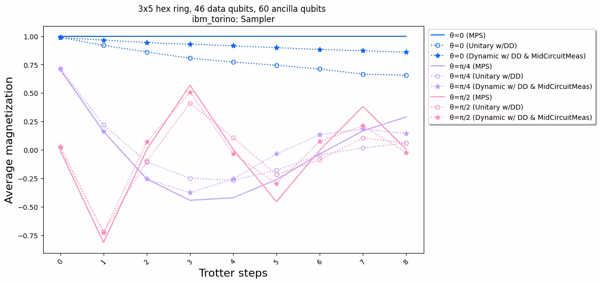
عند مقارنة النتائج التجريبية بالمحاكاة، يتضح أن تطبيق الدوائر الديناميكية (الخط المنقط بالنجوم) يُحقق أداءً أفضل بشكل عام مقارنةً بالتطبيق الأحادي القياسي (الخط المنقط بالدوائر). وخلاصة القول، نقدم الدوائر الديناميكية بوصفها حلاً لمحاكاة نماذج Ising للدوران على شبكة قرص العسل (honeycomb lattice)، وهي طبولوجيا ليست أصيلة في العتاد المادي. يتيح حل الدوائر الديناميكية إجراء تفاعلات ZZ بين كيوبتات غير متجاورة، مع عمق بوابات ثنائية الكيوبت أقصر مما تتطلبه بوابات SWAP، وذلك على حساب إدخال كيوبتات ancilla إضافية وعمليات feedforward كلاسيكية.

المراجع

[1] Quantum computing with Qiskit, by Javadi-Abhari, A., Treinish, M., Krsulich, K., Wood, C.J., Lishman, J., Gacon, J., Martiel, S., Nation, P.D., Bishop, L.S., Cross, A.W. and Johnson, B.R., 2024. arXiv preprint arXiv:2405.08810 (2024)