محاكاة تشتت النيوترونات في المواد الكمومية باستخدام الدوائر الكمومية

تقدير الاستخدام: 13 دقيقة على معالج Heron r2 (ملاحظة: هذا تقدير فقط. قد يختلف وقت التشغيل الفعلي لديك.)

أي درس تعليمي يجب أن أستخدم؟

استخدم هذا الدرس التعليمي لتعلم التنفيذ خطوة بخطوة، مع تشغيل الحساب الكلاسيكي محليًا على حاسوبك المحمول وتنفيذ العتاد على QPU من IBM Quantum®. يتطلب المثال بمقياس كبير ذاكرة كبيرة، ويمكن أن يستغرق التجميع الكمومي التقريبي (AQC) عدة ساعات على موارد حاسوب محمول نموذجية. لنقل الضغط إلى موارد الحوسبة والذاكرة الخاصة بـ Qiskit Serverless، استخدم الدرس التعليمي المصاحب لـ Serverless.

مخرجات التعلم

كيف ترتبط أطياف تشتت النيوترونات غير المرن (INS) بعوامل البنية الديناميكية (DSFs) لنماذج السبين الكمومية.
كيفية تحضير حالة أرضية، وتطبيق اضطراب موضعي، وتنفيذ تطور زمني بتروتر على دائرة كمومية.
كيفية استخدام التجميع الكمومي التقريبي (AQC) مع qiskit-addon-aqc-tensor لضغط دوائر تروتر العميقة من أجل التنفيذ على العتاد.
كيفية استخراج دالة غرين المتأخرة (RGF) من قيم توقع الكيوبت وتحويلها بفورييه إلى DSF.

المتطلبات المسبقة

الخلفية

في هذا الدليل التعليمي، نُعيد إنتاج نتائج Lee et al.، arXiv:2603.15608.

يساعد تشتت النيوترونات الباحثين على توصيف المواد ذات الصلة بالاستدامة، بما في ذلك أقطاب البطاريات. يستكشف هذا البرنامج التعليمي كيف يمكن للدوائر الكمومية محاكاة الإثارات المغناطيسية وربط النماذج النظرية بقياسات التشتت. يطوّر مثال المغناطيس الكمومي فيه أساليب لدراسة سلوك المواد، مساهمًا في مجموعة أدوات البحث الأوسع لاكتشاف المواد.

تشتت النيوترونات غير المرن وعامل البنية الديناميكي

تشتت النيوترونات غير المرن (INS) هو أحد أقوى المسابر التجريبية للإثارات المغناطيسية في المواد الكمومية. عندما تصطدم حزمة من النيوترونات الحرارية أو الباردة ببلورة، تتبادل النيوترونات الفردية كلاً من الزخم $\mathbf{q}$ والطاقة $\omega$ مع النظام الفرعي المغناطيسي. تتناسب شدة التشتت المقاسة مع عامل البنية الديناميكي (DSF)،

$S^{\alpha\beta}(q,\omega) = \sum_{j} e^{-iq\,j}\int_{-\infty}^{\infty} dt\; e^{i\omega t}\, \langle S_0^{\alpha}(0)\, S_j^{\beta}(t)\rangle,$

الذي يُرمّز الارتباطات الكاملة للفضاء والزمن لدرجات حرية السبين.

KCuF $_3$ : مغناطيس نموذجي من نوع سائل لوتينجر

فلوريد النحاس والبوتاسيوم (KCuF $_3$ ) هو مضاد مغناطيسية شبه أحادي البعد تتفاعل فيه سلاسل أيونات Cu $^{2+}$ ذات السبين- $\frac{1}{2}$ عبر تبادل هايزنبرغ لأقرب جار $J$ ، بينما اقتران السلاسل البينية لا يتجاوز $\sim 2.7\%$ من $J$ . عند $T = 6\;\mathrm{K}$ حيث تتوفر بيانات INS، يهيمن على الطيف إثارات سبينون المجزّأة المميزة لسائل تومونجا-لوتينجر. لأن ديناميكيات داخل السلسلة موصوفة جيداً بهاميلتونيان XXZ أحادي البعد ذي السبين- $\frac{1}{2}$ عند النقطة المتماثلة ( $\epsilon = 1$ )،

$H = J\sum_{i}\left[S_i^Z S_{i+1}^Z + \epsilon\left(S_i^X S_{i+1}^X + S_i^Y S_{i+1}^Y\right)\right],$

يُعدّ KCuF $_3$ قياساً مرجعياً مثالياً لمحاكاة الكم: الهاميلتونيان بسيط بما يكفي لتنفيذه على معالج كمومي، ومع ذلك فإن الحالة الأرضية متشابكة بشدة ويتميز طيف الإثارة بمتصل واسع من نوع اثنين-سبينون.

ملاحظة: يضبط هذا الدليل التعليمي $J = 1$ كوحدة طاقة ويعتمد التطبيع $H = J\sum_i[\ldots]$ ، الذي يتوافق مع الهاميلتونيان الموضعي $H_\mathrm{loc} = J(S^X S^X + S^Y S^Y + S^Z S^Z)$ المستخدم في تنفيذ الدائرة في الورقة البحثية (الشكل S3 من المواد التكميلية). الهاميلتونيان الكامل للورقة البحثية (المعادلة 3) يحمل عامل 2 إضافي شامل، لذا فإن $J$ في الورقة البحثية ضعف $J$ المستخدم هنا.

ماذا نُحاكي ونقيس

الكمية الفيزيائية التي نحسبها هي دالة غرين المتأخرة (RGF)، المُعرَّفة كدالة ارتباط سبين-سبين معتمدة على الزمن

$G^R_{\alpha,\beta}(j, j_c, t) = -\frac{i}{2}\,\langle\psi_{\mathrm{GS}}|\,S_j^\alpha(t)\,S_{j_c}^\beta(0) - S_{j_c}^\beta(0)\,S_j^\alpha(t)\,|\psi_{\mathrm{GS}}\rangle,$

حيث $j_c$ هو موقع مرجعي (مركز السلسلة) و $S_j^\alpha(t) = e^{iHt}S_j^\alpha e^{-iHt}$ هو مؤثر السبين في صورة هايزنبرغ. في هذا الدليل التعليمي نركز على المكوّن $zz$ ( $\alpha = \beta = z$ ). على حاسوب كمومي، نحصل على RGF بتحضير الحالة الأرضية، وتطبيق اضطراب موضعي عند $j_c$ ، وتطوير الحالة المضطربة زمنياً، وقياس قيمة توقع الكيوبت المفرد $\langle\sigma_j^z\rangle$ عند كل موقع $j$ لكل خطوة زمنية. الفكرة الأساسية هي أن كل $\langle\sigma_j^z\rangle$ يعطي الفرق عن مغنطة الحالة الأرضية؛ لأن مضاد المغناطيسية هايزنبرغ المتماثل له مغنطة صافية صفرية لكل موقع ( $\langle\sigma_j^z\rangle_\mathrm{GS} = 0$ )، فإن القيمة المقاسة الخام تعطي مباشرة $G^R(j, j_c, t)$ من دون أي طرح صريح.

بجمع $G^R(j, j_c, t)$ عبر جميع المواقع والخطوات الزمنية، نُجمّع مجموعة بيانات ثنائية الأبعاد يتم بعدها تحويلها بفورييه في الفضاء والزمن معاً لإنتاج عامل البنية الديناميكي $S(q,\omega)$ . عامل البنية الديناميكي هو الكمية المقاسة مباشرة في تجربة INS: فهو يخبرنا بالإثارات المغناطيسية الموجودة عند كل زخم $q$ وطاقة $\omega$ . بالنسبة لسلسلة هايزنبرغ المتناحية، فإن طيف الإثارة الدقيق هو متصل اثنين-سبينون، وهو نطاق واسع من شدة التشتت يُستخدم شكله كقياس مرجعي صارم من طرف إلى طرف لمحاكاة الكم: فهو يتحقق من تحضير الحالة الأرضية، والاضطراب، والتطور الزمني بتروتر، وبروتوكول القياس كلها دفعة واحدة.

سير عمل محاكاة الكم

يعكس سير العمل فيزياء حدث INS. نحن (1) نُحضّر الحالة الأرضية متعددة الأجسام $|\psi_{\mathrm{GS}}\rangle$ على $n$ كيوبت، (2) نطبق اضطراب انقلاب سبين موضعياً $U_{j_c} = \frac{1}{\sqrt{2}}(I - i\sigma^z_{j_c})$ في مركز السلسلة لمحاكاة انتقال سبين النيوترون، (3) نُطوّر تحت $H$ لخطوات زمنية منفصلة باستخدام تروتر من الرتبة الثانية، و(4) نقيس $\langle\sigma_i^z\rangle$ على كل كيوبت في كل خطوة للحصول على RGF. ثم يعطي تحويل فورييه المنفصل ثنائي الأبعاد DSF $S(q,\omega)$ .

المرصود (الكمية القابلة للرصد) الذي نقيسه في كل خطوة زمنية هو $\sigma_i^z$ على كل كيوبت $i$ . في Qiskit تُمثَّل هذه كقائمة من مؤثرات SparsePauliOp: مؤثر $Z$ أحادي الكيوبت مُضمَّن في سلسلة الهوية ذات $n$ كيوبت لكل موقع. تُبنى هذه المرصودات مرة واحدة لكل حالة مسألة أثناء خطوة تعيين المسألة (الخطوة 1) وتُعاد استخدامها لكل دائرة على ذلك المقياس.

التجميع الكمومي التقريبي (AQC)

يمكن ضغط دوائر تروتر العميقة باستخدام التجميع الكمومي التقريبي (AQC)، الذي يستبدل عدة طبقات تروتر الأولى بأنساتز مُبارَمتَر أقصر تُحسَّن معاملاته كلاسيكياً لتعظيم الدقة على مستوى MPS مع الدائرة العميقة الأصلية. تُضاف خطوات تروتر المتبقية بشكل دقيق، مُنتجة دائرة "مختلطة" من AQC + تروتر ببوابات ثنائية الكيوبت أقل بشكل كبير.

محاكاة MPS

بالنسبة لنظام أحادي البعد، يمكن لطرق حالة المصفوفة الحاصلية (MPS) أن تُحاكي بكفاءة كلاً من تحضير الحالة الأرضية (باستخدام مجموعة إعادة تسوية مصفوفة الكثافة، أو DMRG) والتطور الزمني على مستوى الدائرة. بالتحكم في بُعد الرابطة $\chi$ ، نُوازن بين الدقة وتكلفة الحوسبة. في هذا الدليل التعليمي نستخدم محاكاة MPS ضمن qiskit-addon-aqc-tensor لحساب أنساتزات AQC عالية الدقة تضغط دوائر تروتر العميقة من أجل التنفيذ على العتاد.

المتطلبات

قبل بدء هذا الدليل التعليمي، تأكد من أن لديك ما يلي مُثبَّتاً:

حزمة Qiskit SDK مع دعم التصور
Qiskit Runtime (pip install qiskit-ibm-runtime)
qiskit-addon-aqc-tensor مع إضافات quimb وJAX (pip install 'qiskit-addon-aqc-tensor[quimb-jax]')

الإعداد

# Added by doQumentation — installs the packages this notebook needs if they are missing
import importlib.util

_needed = {"matplotlib": "matplotlib", "numpy": "numpy", "qiskit": "qiskit", "qiskit_addon_aqc_tensor": "qiskit-addon-aqc-tensor", "qiskit_ibm_runtime": "qiskit-ibm-runtime", "qiskit_quimb": "qiskit-quimb", "quimb": "quimb", "scipy": "scipy"}
_missing = [pip for module, pip in _needed.items()
            if importlib.util.find_spec(module) is None]
# One at a time, so a package that fails to install does not block the others
for _pip in _missing:
    %pip install -q {_pip}
if not _missing:
    print("\u2713 All required packages are installed")

import timeit
import warnings
from collections.abc import Iterator, Sequence
from functools import partial

import matplotlib.pyplot as plt
import numpy as np
import quimb.tensor as qtn
import scipy.optimize
from numpy.typing import NDArray
from qiskit import QuantumCircuit
from qiskit.circuit import CircuitInstruction, ParameterVector, Qubit
from qiskit.circuit.library import PauliEvolutionGate
from qiskit.primitives import StatevectorEstimator
from qiskit.quantum_info import SparsePauliOp
from qiskit.transpiler.preset_passmanagers import generate_preset_pass_manager
from qiskit_addon_aqc_tensor import generate_ansatz_from_circuit
from qiskit_addon_aqc_tensor.objective import MaximizeStateFidelity
from qiskit_addon_aqc_tensor.simulation import tensornetwork_from_circuit
from qiskit_addon_aqc_tensor.simulation.quimb import QuimbSimulator
from qiskit_ibm_runtime import EstimatorV2 as Estimator
from qiskit_ibm_runtime import QiskitRuntimeService
from qiskit_quimb import quimb_circuit
from scipy.sparse import SparseEfficiencyWarning

# scipy.sparse.linalg.expm (reached via PauliEvolutionGate.to_matrix) prefers
# CSC and warns when handed the CSR matrix from SparsePauliOp.to_matrix; the
# result is unaffected, so silence the cosmetic warning.
warnings.filterwarnings("ignore", category=SparseEfficiencyWarning)

def xxz_hamiltonian_mpo(
    n_qubits: int, interaction: float = 1.0, anisotropy: float = 1.0
) -> qtn.MatrixProductOperator:
    """1D XXZ Hamiltonian as a quimb MPO.

    Builds the Hamiltonian using ``qtn.SpinHam1D``.

    Args:
        n_qubits: Number of sites.
        interaction: Overall interaction strength (J in the paper).
        anisotropy: XY/Z anisotropy (ε in the paper). ``ε = 1`` is the
            isotropic Heisenberg point; ``ε = 0`` is the Ising limit.

    Returns:
        The Hamiltonian as a matrix product operator.
    """
    builder = qtn.SpinHam1D(S=1 / 2)
    builder += interaction * anisotropy * 0.5, "+", "-"
    builder += interaction * anisotropy * 0.5, "-", "+"
    builder += interaction, "Z", "Z"
    return builder.build_mpo(L=n_qubits)

def build_ground_state_ansatz(n_qubits: int, n_layers: int) -> QuantumCircuit:
    """Hamiltonian variational ansatz (HVA) circuit for ground-state preparation.

    Starts from a product of singlet pairs and applies alternating
    odd/even layers of parameterized XXZ pair-evolution gates.

    The returned circuit is parameterized: it carries a ``ParameterVector``
    named ``"theta"`` of length ``2 * n_layers`` whose values must be
    assigned (e.g. via ``circuit.assign_parameters``) before simulation.
    Element ``2 * r`` is the odd-layer angle and element ``2 * r + 1`` is the
    even-layer angle of layer ``r``.

    Args:
        n_qubits: Number of qubits (must be even).
        n_layers: Number of HVA layers.

    Returns:
        The parameterized HVA preparation circuit.
    """
    theta = ParameterVector("theta", 2 * n_layers)
    circuit = QuantumCircuit(n_qubits)
    # Initial singlet product state
    for i in range(n_qubits // 2):
        circuit.x(2 * i)
        circuit.x(2 * i + 1)
        circuit.h(2 * i + 1)
        circuit.cx(2 * i + 1, 2 * i)
    # Variational layers: each pair gate is exp(-i theta (XX+YY+ZZ)/2)
    pair_ham = SparsePauliOp(
        ["XX", "YY", "ZZ"], coeffs=[0.5, 0.5, 0.5]
    )  # H_pair (HVA form)
    for r in range(n_layers):
        for i in range(1, (n_qubits + 1) // 2):  # odd layer
            circuit.append(
                PauliEvolutionGate(pair_ham, time=theta[2 * r]),
                [2 * i - 1, 2 * i],
            )
        for i in range(n_qubits // 2):  # even layer
            circuit.append(
                PauliEvolutionGate(pair_ham, time=theta[2 * r + 1]),
                [2 * i, 2 * i + 1],
            )
    return circuit

def optimize_ground_state_ansatz(
    ansatz: QuantumCircuit,
    x0: NDArray[np.floating],
    target_mps: qtn.MatrixProductState,
    *,
    max_bond: int | None = None,
    cutoff: float = 1e-10,
    method: str = "COBYQA",
    options: dict | None = None,
) -> scipy.optimize.OptimizeResult:
    """Optimize HVA parameters by maximizing fidelity with a target MPS.

    The HVA circuit is simulated as a matrix product state with the given
    bond-dimension truncation, and the parameters are optimized to maximize
    the state fidelity ``|<psi_HVA | target_mps>|**2`` with the DMRG ground
    state. Both states are normalized, so the minimized objective is the
    infidelity ``1 - |<psi_HVA | target_mps>|**2``.

    Args:
        ansatz: Parameterized HVA circuit from ``build_ground_state_ansatz``.
            The length of ``x0`` must equal ``ansatz.num_parameters``.
        x0: Initial parameters.
        target_mps: Target MPS (DMRG ground state) to maximize fidelity with.
        max_bond: Maximum MPS bond dimension during gate application.
        cutoff: Singular-value cutoff during gate application.
        method: ``scipy.optimize.minimize`` method.
        options: Options dict forwarded to ``scipy.optimize.minimize``.

    Returns:
        The Scipy OptimizeResult.
    """

    def infidelity(params: NDArray[np.floating]) -> float:
        circuit = ansatz.assign_parameters(params)
        circuit_mps = quimb_circuit(
            circuit.decompose(["PauliEvolution"]),
            quimb_circuit_class=qtn.CircuitMPS,
            max_bond=max_bond,
            cutoff=cutoff,
        )
        return 1 - abs(circuit_mps.psi.H @ target_mps) ** 2

    return scipy.optimize.minimize(
        infidelity, np.asarray(x0), method=method, options=options
    )

def trotter_evolution(
    qubits: Sequence[Qubit],
    interaction: float,
    anisotropy: float,
    time_step: float,
    n_steps: int,
) -> Iterator[CircuitInstruction]:
    """Second-order Trotter steps of the XXZ pair Hamiltonian.

    While the paper used a hand-optimized circuit for the Trotter steps, we use
    PauliEvolutionGate here for simplicity and generality. The final two-qubit gate
    count and gate depth are equivalent when transpiled with ``optimization_level=3``.

    Args:
        qubits: Qubits to act on (length ``n_qubits``).
        interaction: Overall interaction strength (J in the paper).
        anisotropy: XY/Z anisotropy (ε in the paper). ``ε = 1`` is the
            isotropic Heisenberg point; ``ε = 0`` is the Ising limit.
        time_step: Per-step Trotter time.
        n_steps: Number of Trotter steps.

    Yields:
        ``CircuitInstruction``s implementing the Trotter steps.
    """
    if n_steps == 0:
        return
    n_qubits = len(qubits)
    pair_ham = SparsePauliOp(
        ["XX", "YY", "ZZ"],
        coeffs=[
            0.25 * interaction * anisotropy,
            0.25 * interaction * anisotropy,
            0.25 * interaction,
        ],
    )
    half_evo = PauliEvolutionGate(pair_ham, time=time_step / 2)
    full_evo = PauliEvolutionGate(pair_ham, time=time_step)
    for i in range(n_qubits // 2):  # half even layer
        yield CircuitInstruction(half_evo, (qubits[2 * i], qubits[2 * i + 1]))
    for i in range(n_qubits // 2 - 1):  # full odd layer
        yield CircuitInstruction(
            full_evo, (qubits[2 * i + 1], qubits[2 * i + 2])
        )
    for _ in range(n_steps - 1):  # interior steps
        for i in range(n_qubits // 2):
            yield CircuitInstruction(
                full_evo, (qubits[2 * i], qubits[2 * i + 1])
            )
        for i in range(n_qubits // 2 - 1):
            yield CircuitInstruction(
                full_evo, (qubits[2 * i + 1], qubits[2 * i + 2])
            )
    for i in range(n_qubits // 2):  # half even layer
        yield CircuitInstruction(half_evo, (qubits[2 * i], qubits[2 * i + 1]))

def get_dsf(
    n_qubits: int,
    rgf_mat: NDArray[np.floating],
    time_step: float,
    n_steps: int,
    n_points_momentum: int,
    n_points_frequency: int,
) -> NDArray[np.floating]:
    """Compute the dynamical structure factor from the retarded Green's function.

    Uses the center-site approximation and a discrete Fourier transform.
    The result is symmetrized about the momentum axis and clipped to
    non-negative values, ready for plotting.

    Args:
        n_qubits: Number of qubits (sites).
        rgf_mat: RGF matrix of shape ``(n_steps, n_qubits)``.
        time_step: Trotter time-step size.
        n_steps: Number of time steps.
        n_points_momentum: Number of momentum points.
        n_points_frequency: Number of frequency points.

    Returns:
        DSF array of shape ``(n_points_frequency, n_points_momentum)``,
        symmetrized about the momentum axis and clipped to non-negative values.
    """
    max_frequency = np.pi / time_step
    momentum_range = np.linspace(0, 2 * np.pi, n_points_momentum)
    frequency_range = np.linspace(0, max_frequency, n_points_frequency)
    result = np.zeros((frequency_range.shape[0], momentum_range.shape[0]))
    center = n_qubits // 2 - 1
    for iw, w in enumerate(frequency_range):
        exponent = np.exp(1j * w * time_step * np.arange(1, n_steps + 1))
        # S = sigma/2, so two spin operators contribute a factor of (1/2)(1/2) = 1/4.
        rgf_omega = (
            np.dot(rgf_mat.T, exponent) * time_step / 4
        )  # S(omega): time Fourier slice of the Green's function
        for iq, q in enumerate(momentum_range):
            momentum_phases = np.exp(
                -1j * q * np.arange(-center, center + 2, 1)
            )
            result[iw, iq] = np.imag(np.dot(rgf_omega, momentum_phases))
    result = -(result + result[:, ::-1]) / 2
    result = np.clip(result, a_min=0, a_max=None)
    return result

def plot_dsf(
    dsf: NDArray[np.floating],
    time_step: float,
    n_points_momentum: int,
    n_points_frequency: int,
    title: str | None = None,
) -> None:
    """Heat-map of the dynamical structure factor.

    Args:
        dsf: DSF array of shape ``(n_points_frequency, n_points_momentum)``.
        time_step: Trotter time-step size.
        n_points_momentum: Number of momentum points.
        n_points_frequency: Number of frequency points.
        title: Optional plot title.
    """
    max_frequency = np.pi / time_step
    momentum_range = np.linspace(0, 2 * np.pi, n_points_momentum)
    frequency_range = np.linspace(0, max_frequency, n_points_frequency)
    x, y = np.meshgrid(momentum_range, frequency_range)
    fig, ax = plt.subplots(figsize=(8, 5))
    c = ax.pcolormesh(x, y, dsf / np.max(dsf), cmap="viridis", shading="auto")
    fig.colorbar(c, ax=ax, label="Normalized intensity")
    ax.set_ylim(0, 3.6)
    ax.set_xlim(0, 2 * np.pi)
    ax.set_xlabel(r"$q$", fontsize=16)
    ax.set_ylabel(r"$\tilde{\omega} = \omega / J$", fontsize=16)
    ax.set_xticks([0, np.pi / 2, np.pi, 3 * np.pi / 2, 2 * np.pi])
    ax.set_xticklabels(["0", r"$\pi/2$", r"$\pi$", r"$3\pi/2$", r"$2\pi$"])
    if title:
        ax.set_title(title, fontsize=14)
    plt.tight_layout()
    plt.show()

def plot_rgf(
    n_qubits: int,
    rgf_mat: NDArray[np.floating],
    time_step: float,
    n_steps: int,
    title: str | None = None,
) -> None:
    """Heat-map of the retarded Green's function in real space and time.

    Args:
        n_qubits: Number of qubits (sites).
        rgf_mat: RGF matrix of shape ``(n_steps, n_qubits)``.
        time_step: Trotter time-step size.
        n_steps: Number of time steps.
        title: Optional plot title.
    """
    fig, ax = plt.subplots(figsize=(8, 6))
    qubit_axis = np.arange(n_qubits)
    t_axis = np.arange(1, n_steps + 1) * time_step
    x, y = np.meshgrid(qubit_axis, t_axis)
    c = ax.pcolormesh(
        x,
        y,
        np.real(rgf_mat),
        cmap="RdBu",
        vmax=0.5,
        vmin=-0.5,
        shading="auto",
    )
    fig.colorbar(c, ax=ax, label=r"Re $G^R(j, j_c, t)$")
    ax.set_xlabel("Qubit", fontsize=16)
    ax.xaxis.set_major_locator(
        plt.matplotlib.ticker.MaxNLocator(integer=True)
    )
    ax.set_ylabel(r"Time", fontsize=16)
    if title:
        ax.set_title(title, fontsize=14)
    plt.tight_layout()
    plt.show()

def uniform_2q_depth(circuit: QuantumCircuit) -> int:
    """Two-qubit gate depth in a standardized basis."""
    pass_manager = generate_preset_pass_manager(
        optimization_level=0, basis_gates=["cz", "id", "rz", "sx", "x"]
    )
    return pass_manager.run(circuit).depth(
        lambda inst: inst.operation.num_qubits == 2
    )

مثال محاكي صغير المقياس

نُظهر أولاً سير العمل الكامل على 10 كيوبتات، مع تحسين أنساتز الحالة الأرضية HVA باستخدام محاكاة MPS واستخدام محاكي متجه الحالة في Qiskit للتطور الزمني. يعطي DMRG طاقة حالة أرضية مرجعية وMPS مرجعياً. يتيح لنا هذا المثال صغير المقياس التحقق من كل خطوة قبل التوسع.

الخطوة 1: تعيين المدخلات الكلاسيكية إلى مسألة كمومية

نبدأ بتعريف النموذج الفيزيائي وبناء الدوائر الكمومية.

الهاميلتونيان. يُنمذج KCuF $_3$ بهاميلتونيان XXZ أحادي البعد عند النقطة المتناحية ( $J = 1$ ، $\epsilon = 1$ ، بضبط $J = 1$ كوحدة طاقة).

الحالة الأرضية. نستخدم دائرة أنساتز تبايُني للهاميلتونيان (HVA)، build_ground_state_ansatz، كدائرة تحضير الحالة الأرضية. تُحسَّن معاملات HVA كلاسيكياً بتعظيم أمانة الحالة $|\langle\psi_{\mathrm{HVA}}(\theta)|\psi_{\mathrm{DMRG}}\rangle|^2$ مع MPS للحالة الأرضية من DMRG، حيث تُقيَّم حالة HVA بمحاكاة الدائرة كحالة مصفوفة حاصلية باستخدام CircuitMPS من quimb. نستخدم scipy.optimize.minimize للتحسين. تُحسب أيضاً طاقة $\langle H \rangle$ للأنساتز المُحسَّن للمرجعية.

بوابات تروتر. يُبنى كل حد تفاعل لأقرب جار $e^{-i\Delta t\, H_{\mathrm{pair}}}$ مع $H_{\mathrm{pair}} = (J/4)(XX + YY + ZZ)$ باستخدام PauliEvolutionGate(H_pair, time=time_step). يُحلّل Qiskit هذا إلى تفكيك ثلاثي CNOT الأمثل أثناء الترجمة.

الاضطراب. بوابة $R_z(\pi/2)$ على الكيوبت المركزي تُنفّذ $U_{j_c} = \frac{1}{\sqrt{2}}(I - i\sigma^z_{j_c})$ ، محاكيةً انقلاب السبين الموضعي الناتج عن نيوترون متشتت.

الملاحظات. نبني ملاحظة $\sigma^z$ لكل موقع كيوبت. تُمرَّر كائنات SparsePauliOp هذه إلى أولية Estimator في الخطوة 3 لاستخراج $\langle\sigma_i^z\rangle$ في كل خطوة زمنية.

# -- Physical parameters --
n_qubits = 10
interaction = 1.0  # J
anisotropy = 1.0  # ε (isotropic point)
time_step = 0.6
n_steps = 10
mps_max_bond = 32
mps_cutoff = 1e-8
center = n_qubits // 2 - 1

# -- Hamiltonian MPO --
ham_mpo = xxz_hamiltonian_mpo(n_qubits, interaction, anisotropy)

# -- Reference ground-state energy via DMRG --
dmrg = qtn.DMRG2(ham_mpo)
dmrg.solve(tol=1e-8)
print(f"Ground-state energy (DMRG): {dmrg.energy:.6f}")

# -- Build ground state ansatz circuit --
gs_n_layers = 3
gs_ansatz = build_ground_state_ansatz(n_qubits, gs_n_layers)

# -- Optimize ground state ansatz parameters to maximize fidelity with the DMRG MPS --
# Initialize odd-layer angles near 0 (where the inter-pair gate is the
# identity) and even-layer angles near pi/2 (where the intra-pair gate
# is a SWAP, since 0.5*(XX + YY + ZZ) = SWAP - I/2).
rng = np.random.default_rng(12345)
x0 = np.tile([0, np.pi / 2], gs_n_layers) + rng.normal(
    scale=0.1, size=2 * gs_n_layers
)
print("Optimizing ground state ansatz...")
t0 = timeit.default_timer()
result = optimize_ground_state_ansatz(
    gs_ansatz,
    x0,
    dmrg.state,
    max_bond=mps_max_bond,
    cutoff=mps_cutoff,
    options=dict(maxiter=100),
)
t1 = timeit.default_timer()
print(f"Finished optimizing ground state ansatz in {t1 - t0} seconds.")
print(f"Ground state ansatz fidelity: {1 - result.fun:.6f}")

gs_circuit = gs_ansatz.assign_parameters(result.x)
gs_circuit_mps = quimb_circuit(
    gs_circuit.decompose(["PauliEvolution"]),
    quimb_circuit_class=qtn.CircuitMPS,
    max_bond=mps_max_bond,
    cutoff=mps_cutoff,
)
gs_ansatz_energy = qtn.expec_TN_1D(
    gs_circuit_mps.psi.H, ham_mpo, gs_circuit_mps.psi
)
print(f"Ground state ansatz energy: {gs_ansatz_energy:.6f}")

# -- Build circuits for each time step --
perturbed = gs_circuit.copy()
perturbed.rz(np.pi / 2, center)

circuits = []
for t in range(1, n_steps + 1):
    circuit = perturbed.copy()
    for instr in trotter_evolution(
        circuit.qubits, interaction, anisotropy, time_step, t
    ):
        circuit.append(instr)
    circuits.append(circuit)
print(
    f"Built {len(circuits)} circuits, deepest 2q depth (uniform basis) = "
    f"{uniform_2q_depth(circuits[-1])}"
)

# -- Observables: Z on each qubit site --
observables = [
    SparsePauliOp.from_sparse_list([("Z", [i], 1)], num_qubits=n_qubits)
    for i in range(n_qubits)
]
print(f"Defined {len(observables)} Z observables.")

Ground-state energy (DMRG): -4.258035
Optimizing ground state ansatz...
Finished optimizing ground state ansatz in 8.850687621976249 seconds.
Ground state ansatz fidelity: 0.984277
Ground state ansatz energy: -4.232565
Built 10 circuits, deepest 2q depth (uniform basis) = 163
Defined 10 Z observables.

الخطوة 2: تحسين المسألة لتنفيذها على العتاد الكمومي

بالنسبة للعتاد الحقيقي، ستكون دوائر تروتر أعلاه عميقة جداً. يُعالج التجميع الكمومي التقريبي (AQC) هذا باستبدال أول $k$ طبقة تروتر (بما فيها دائرة الحالة الأرضية) بأنساتز مُبارَمتَر أقصر مُحسَّن لتعظيم الدقة على مستوى MPS مع الدائرة العميقة الأصلية. تُضاف خطوات تروتر المتبقية بشكل دقيق، مُنتجة دائرة "AQC + تروتر" أقل عمقاً.

لموازنة قابلية التعبير مقابل عمق الدائرة، يُستخدم أنساتزان: أنساتز بطبقة واحدة (مولّد من خطوة تروتر واحدة) يضغط الخطوات الزمنية الأولى، وأنساتز أعمق بطبقتين (مولّد من خطوتي تروتر) يضغط الخطوات القليلة التالية حيث تُحتاج أمانة أعلى.

يتكون سير عمل AQC من أربع خطوات فرعية:

بناء الدوائر الهدف — أول $k_1 + k_2$ دائرة من الخطوة 1 تُستخدم مباشرة كأهداف AQC.
حساب MPS الهدف — محاكاة كل دائرة هدف كحالة مصفوفة حاصلية باستخدام quimb.tensor.CircuitMPS.
توليد وتحسين الأنساتزات — generate_ansatz_from_circuit يُنشئ أنساتز بطبقة واحدة وأنساتز بطبقتين؛ تُحسَّن المعاملات باستخدام L-BFGS-B مع تدرجات مُسرَّعة بـ JAX لتقليل $1 - |\langle\psi_{\mathrm{ansatz}}|\psi_{\mathrm{target}}\rangle|^2$ . تستخدم أول $k_1$ خطوة الأنساتز ذا الطبقة الواحدة والـ $k_2$ خطوة التالية الأنساتز ذا الطبقتين؛ ضمن كل مرحلة، تبدأ كل خطوة بشكل دافئ من المعاملات المُحسَّنة للخطوة السابقة، وتُعاد المعاملات إلى الافتراضيات عند حدود المرحلة.
تجميع الدوائر المختلطة — بالنسبة للخطوات الزمنية بعد نقطة تفتيش AQC، تُضاف طبقات تروتر الدقيقة إلى دائرة AQC ذات الطبقتين المُحسَّنة باستخدام trotter_evolution.

# Number of time steps to compress into an AQC ansatz with one layer
aqc_n_steps_1 = 3
# Number of time steps to compress into an AQC ansatz with two layers
aqc_n_steps_2 = 2
aqc_n_steps_total = aqc_n_steps_1 + aqc_n_steps_2

# ── Step 2a: Target circuits (first aqc_n_steps_total circuits from Step 1) ──
target_circuits = {
    k: circuits[k - 1] for k in range(1, aqc_n_steps_total + 1)
}
# ── Step 2b: Compute target MPS ──
# Decompose PauliEvolutionGate to RXX/RYY/RZZ before passing to the AQC MPS
# backend, which does not understand PauliEvolutionGate natively.
aqc_sim = QuimbSimulator(
    quimb_circuit_factory=partial(
        qtn.CircuitMPS,
        gate_opts=dict(max_bond=mps_max_bond, cutoff=mps_cutoff),
    ),
    autodiff_backend="jax",
)
print("\nStep 2b — target MPS:")
target_mps = {}
for k in range(1, aqc_n_steps_total + 1):
    target_mps[k] = tensornetwork_from_circuit(
        target_circuits[k].decompose(["PauliEvolution"]), aqc_sim
    )
    print(f"  k={k}: max bond = {target_mps[k].psi.max_bond()}")

# ── Step 2c: Generate ansätze (one-layer and two-layer) and optimize parameters ──
ansatz_1, initial_params_1 = generate_ansatz_from_circuit(
    target_circuits[1].decompose(["PauliEvolution"]),
    qubits_initially_zero=True,
)
initial_params_1 = np.array(initial_params_1)
ansatz_2, initial_params_2 = generate_ansatz_from_circuit(
    target_circuits[2].decompose(["PauliEvolution"]),
    qubits_initially_zero=True,
)
initial_params_2 = np.array(initial_params_2)
print(
    f"\nStep 2c — one-layer ansatz: {ansatz_1.num_parameters} parameters, "
    f"2q depth (uniform basis) = {uniform_2q_depth(ansatz_1)}"
)
print(
    f"Step 2c — two-layer ansatz: {ansatz_2.num_parameters} parameters, "
    f"2q depth (uniform basis) = {uniform_2q_depth(ansatz_2)}"
)

aqc_circuits = {}
aqc_params = {}
for k in range(1, aqc_n_steps_total + 1):
    if k <= aqc_n_steps_1:
        ansatz, base_params = ansatz_1, initial_params_1
    else:
        ansatz, base_params = ansatz_2, initial_params_2
    # Warm-start from the previous step only within the same stage
    same_stage = (k - 1 >= 1) and (
        (k - 1 <= aqc_n_steps_1) == (k <= aqc_n_steps_1)
    )
    x0 = aqc_params[k - 1] if same_stage else base_params
    obj = MaximizeStateFidelity(target_mps[k], ansatz, aqc_sim)
    t0 = timeit.default_timer()
    result = scipy.optimize.minimize(
        obj.loss_function,
        x0,
        method="L-BFGS-B",
        jac=True,
        options=dict(maxiter=100),
    )
    elapsed = timeit.default_timer() - t0
    aqc_params[k] = result.x
    aqc_circuits[k] = ansatz.assign_parameters(result.x)
    print(
        f"  k={k}: fidelity = {1 - result.fun:.4f}, "
        f"2q depth (uniform basis) = "
        f"{uniform_2q_depth(aqc_circuits[k])}, "
        f"{elapsed:.1f}s"
    )

# ── Step 2d: Assemble full circuit set (AQC + Trotter) ──
all_circuits = []
for k in range(1, aqc_n_steps_total + 1):
    all_circuits.append(aqc_circuits[k])
base = aqc_circuits[aqc_n_steps_total]
for k in range(1, n_steps - aqc_n_steps_total + 1):
    circuit = base.copy()
    for instr in trotter_evolution(
        circuit.qubits, interaction, anisotropy, time_step, k
    ):
        circuit.append(instr)
    all_circuits.append(circuit)

full_depths = [
    uniform_2q_depth(circuits[k - 1]) for k in range(1, n_steps + 1)
]
aqc_depths = [uniform_2q_depth(circuit) for circuit in all_circuits]
full_2q = [
    circuits[k - 1].decompose(["PauliEvolution"]).num_nonlocal_gates()
    for k in range(1, n_steps + 1)
]
aqc_2q = [
    circuit.decompose(["PauliEvolution"]).num_nonlocal_gates()
    for circuit in all_circuits
]
print(f"\nStep 2d — assembled {len(all_circuits)} circuits")
print(
    f"  At step {n_steps} (uniform basis): "
    f"Trotter 2q depth = {full_depths[-1]}, AQC+Trotter 2q depth = {aqc_depths[-1]}; "
    f"2q gates: Trotter = {full_2q[-1]}, AQC+Trotter = {aqc_2q[-1]}"
)

steps_axis = np.arange(1, n_steps + 1)
fig, ax = plt.subplots(figsize=(7, 4))
ax.plot(steps_axis, full_depths, "-o", color="black", label="Full Trotter")
ax.plot(
    steps_axis, aqc_depths, "-o", color="cadetblue", label="AQC + Trotter"
)
ax.set_xlabel("Trotter steps", fontsize=13)
ax.xaxis.set_major_locator(plt.matplotlib.ticker.MaxNLocator(integer=True))
ax.set_ylabel("2q gate depth (uniform basis)", fontsize=13)
ax.set_title(f"AQC circuit-depth reduction ({n_qubits} qubits)", fontsize=13)
ax.legend(fontsize=11)
plt.tight_layout()
plt.show()

Step 2b — target MPS:
  k=1: max bond = 22
  k=2: max bond = 22
  k=3: max bond = 26
  k=4: max bond = 27
  k=5: max bond = 30

Step 2c — one-layer ansatz: 389 parameters, 2q depth (uniform basis) = 27
Step 2c — two-layer ansatz: 470 parameters, 2q depth (uniform basis) = 33
  k=1: fidelity = 1.0000, 2q depth (uniform basis) = 27, 11.8s
  k=2: fidelity = 0.9980, 2q depth (uniform basis) = 27, 13.2s
  k=3: fidelity = 0.9890, 2q depth (uniform basis) = 27, 13.7s
  k=4: fidelity = 0.9983, 2q depth (uniform basis) = 33, 16.4s
  k=5: fidelity = 0.9957, 2q depth (uniform basis) = 33, 16.4s

Step 2d — assembled 10 circuits
  At step 10 (uniform basis): Trotter 2q depth = 163, AQC+Trotter 2q depth = 99; 2q gates: Trotter = 371, AQC+Trotter = 200

Output of the previous code cell

الخطوة 3: التنفيذ باستخدام أوليات Qiskit

نُحاكي كل دائرة مُجمَّعة بـ AQC باستخدام أولية StatevectorEstimator.

estimator = StatevectorEstimator()
pubs = [(circuit, observables) for circuit in all_circuits]
job = estimator.run(pubs)
result = job.result()

الخطوة 4: معالجة النتيجة بعد الحصول عليها وإعادتها بالشكل الكلاسيكي المطلوب

نستخرج الآن قيمة التوقع $\langle\sigma_i^z\rangle$ لكل كيوبت $i$ في كل خطوة زمنية $t$ . تُشكّل هذه القيم مصفوفة دالة غرين المتأخرة $G^R(j, j_c, t)$ . ثم نحوّل RGF بفورييه إلى عامل البنية الديناميكي $S(q, \omega)$ ونرسم كلاً من RGF وDSF. تُطبّق get_dsf التماثل المرآتي وتقص القيم السالبة داخلياً.

rgf_mat = np.stack([pub_result.data.evs for pub_result in result])

# -- Compute DSF --
n_points_momentum, n_points_frequency = 100, 100
spectrum = get_dsf(
    n_qubits,
    rgf_mat,
    time_step,
    n_steps,
    n_points_momentum,
    n_points_frequency,
)

# -- Plot retarded Green's function --
plot_rgf(
    n_qubits,
    rgf_mat,
    time_step,
    n_steps,
    title=f"Retarded Green's function — {n_qubits} qubits (simulation)",
)

# -- Plot DSF --
plot_dsf(
    spectrum,
    time_step,
    n_points_momentum,
    n_points_frequency,
    title=f"Dynamical structure factor — {n_qubits} qubits (simulation)",
)

Output of the previous code cell

التنفيذ العتادي واسع النطاق

نتوسع الآن إلى 50 كيوبتاً. عند هذا المقياس، تصل التحسينات إلى أمانة أقل من مثال المقياس الصغير: تنخفض أمانة أنساتز الحالة الأرضية إلى حوالي 0.65، وتنخفض أمانة AQC إلى حوالي 0.7 عند نقاط التفتيش المتأخرة. هذا متوقع، ويمكنك تحسين هذه الأمانة بزيادة عدد طبقات أنساتز الحالة الأرضية (gs_n_layers) أو عدد تكرارات التحسين (maxiter) بتكلفة كلاسيكية إضافية. لاحظ أيضاً أن أمانة AQC ذات الطبقتين تأتي أقل من تلك ذات الطبقة الواحدة. هذا ليس تراجعاً: الخطوات الزمنية المتأخرة تُولّد تشابكاً أكبر وهي أصعب في الضغط، وهذا هو سبب استخدام الأنساتز الأكثر تعبيراً بطبقتين لها.

يمكن أن يستغرق تحسين AQC أيضاً عدة ساعات من وقت الحوسبة الكلاسيكية (حوالي ست ساعات في التشغيل الموضح هنا، أُنفق معظمها على نقاط تفتيش الطبقتين في الخطوة 2c). لتقليل الوقت الفعلي، فكّر في تشغيل دفتر الملاحظات هذا على عتاد كلاسيكي أقوى، مثل نظام حوسبة عالي الأداء (HPC). بدلاً من ذلك، يمكنك تقليص المسألة إلى حالة أصغر (على سبيل المثال، عدد أقل من الكيوبتات أو الخطوات الزمنية)؛ ستختلف نتائجك حينها عن تلك الموضحة هنا.

يتبع الكود أدناه نفس بنية الخطوات الأربع كما في المثال صغير المقياس. تُحسَّن معاملات الحالة الأرضية HVA مرة أخرى باستخدام محاكاة MPS. على QPU، نُفعّل فك الاقتران الديناميكي (DD)، وتمويه باولي، وإخماد خطأ القراءة المموّه (TREX) للقمع والتخفيف من الأخطاء. يلخّص الجدول التالي كيف تختلف التجربة واسعة النطاق عن التجربة صغيرة النطاق:

	مقياس صغير	مقياس كبير
الكيوبتات	10	50
الخطوات الزمنية	10	20
نقاط تفتيش AQC (طبقة واحدة + طبقتان)	3 + 2 = 5	6 + 4 = 10
طبقات أنساتز الحالة الأرضية	3	5
أقصى بُعد رابطة MPS	32	128
Estimator	`StatevectorEstimator`	QPU مع DD وتمويه باولي وTREX

رسائل بطء تجميع XLA

أثناء تحسين AQC (الخطوة 2c أدناه) قد ترى رسائل stderr مثل:

[Compiling module jit_MakeArrayFn for CPU] Very slow compile? ...
The operation took 2m14s

هذه تشخيصات غير ضارة من XLA، المُجمّع الذي يدعم التفاضل التلقائي بـ JAX في qiskit-addon-aqc-tensor. عند 50 كيوبتاً مع بُعد رابطة MPS يساوي 128، يقضي XLA بضع دقائق في تجميع دالة التدرج أول مرة يُتتبّع فيها. ينجح التجميع، ولا تتأثر نتائج التحسين.

# ── Parameters ──────────────────────────────────────────────────────────────
n_qubits = 50  # 10 → 50
interaction = 1.0  # J
anisotropy = 1.0  # ε (isotropic point)
time_step = 0.6
n_steps = 20  # 10 → 20
aqc_n_steps_1 = 6  # 3 → 6
aqc_n_steps_2 = 4  # 2 → 4
aqc_n_steps_total = aqc_n_steps_1 + aqc_n_steps_2
gs_n_layers = 5  # 3 → 5
mps_max_bond = 128  # 32 -> 128
mps_cutoff = 1e-8
center = n_qubits // 2 - 1

# ── Step 1: Map ──────────────────────────────────────────────────────────────
ham_mpo = xxz_hamiltonian_mpo(n_qubits, interaction, anisotropy)

dmrg = qtn.DMRG2(ham_mpo)
dmrg.solve(tol=1e-8)
print(f"Ground-state energy (DMRG): {dmrg.energy:.6f}")

gs_ansatz = build_ground_state_ansatz(n_qubits, gs_n_layers)

rng = np.random.default_rng(12345)
x0 = np.tile([0.0, np.pi / 2], gs_n_layers) + rng.normal(
    scale=0.1, size=2 * gs_n_layers
)
print("Optimizing ground state ansatz...")
t0 = timeit.default_timer()
result = optimize_ground_state_ansatz(
    gs_ansatz,
    x0,
    dmrg.state,
    max_bond=mps_max_bond,
    cutoff=mps_cutoff,
    options=dict(maxiter=100),
)
t1 = timeit.default_timer()
print(f"Finished optimizing ground state ansatz in {t1 - t0} seconds.")
print(f"Ground state ansatz fidelity: {1 - result.fun:.6f}")

gs_circuit = gs_ansatz.assign_parameters(result.x)
gs_circuit_mps = quimb_circuit(
    gs_circuit.decompose(["PauliEvolution"]),
    quimb_circuit_class=qtn.CircuitMPS,
    max_bond=mps_max_bond,
    cutoff=mps_cutoff,
)
gs_ansatz_energy = qtn.expec_TN_1D(
    gs_circuit_mps.psi.H, ham_mpo, gs_circuit_mps.psi
)
print(f"Ground state ansatz energy: {gs_ansatz_energy:.6f}")

perturbed = gs_circuit.copy()
perturbed.rz(np.pi / 2, center)

circuits = []
for t in range(1, n_steps + 1):
    circuit = perturbed.copy()
    for instr in trotter_evolution(
        circuit.qubits, interaction, anisotropy, time_step, t
    ):
        circuit.append(instr)
    circuits.append(circuit)
print(
    f"Built {len(circuits)} circuits, deepest 2q depth (uniform basis) = "
    f"{uniform_2q_depth(circuits[-1])}"
)

observables = [
    SparsePauliOp.from_sparse_list([("Z", [i], 1)], num_qubits=n_qubits)
    for i in range(n_qubits)
]
print(f"Defined {len(observables)} Z observables.")

# ── Step 2: AQC ──────────────────────────────────────────────────────────────
target_circuits = {
    k: circuits[k - 1] for k in range(1, aqc_n_steps_total + 1)
}

aqc_sim = QuimbSimulator(
    quimb_circuit_factory=partial(
        qtn.CircuitMPS,
        gate_opts=dict(max_bond=mps_max_bond, cutoff=mps_cutoff),
    ),
    autodiff_backend="jax",
)
print("\nStep 2b — target MPS:")
target_mps = {}
for k in range(1, aqc_n_steps_total + 1):
    target_mps[k] = tensornetwork_from_circuit(
        target_circuits[k].decompose(["PauliEvolution"]), aqc_sim
    )
    print(f"  k={k}: max bond = {target_mps[k].psi.max_bond()}")

ansatz_1, initial_params_1 = generate_ansatz_from_circuit(
    target_circuits[1].decompose(["PauliEvolution"]),
    qubits_initially_zero=True,
)
initial_params_1 = np.array(initial_params_1)
ansatz_2, initial_params_2 = generate_ansatz_from_circuit(
    target_circuits[2].decompose(["PauliEvolution"]),
    qubits_initially_zero=True,
)
initial_params_2 = np.array(initial_params_2)
print(
    f"\nStep 2c — one-layer ansatz: {ansatz_1.num_parameters} parameters, "
    f"2q depth (uniform basis) = {uniform_2q_depth(ansatz_1)}"
)
print(
    f"Step 2c — two-layer ansatz: {ansatz_2.num_parameters} parameters, "
    f"2q depth (uniform basis) = {uniform_2q_depth(ansatz_2)}"
)

aqc_circuits = {}
aqc_params = {}
for k in range(1, aqc_n_steps_total + 1):
    if k <= aqc_n_steps_1:
        ansatz, base_params = ansatz_1, initial_params_1
    else:
        ansatz, base_params = ansatz_2, initial_params_2
    # Warm-start from the previous step only within the same stage
    same_stage = (k - 1 >= 1) and (
        (k - 1 <= aqc_n_steps_1) == (k <= aqc_n_steps_1)
    )
    x0 = aqc_params[k - 1] if same_stage else base_params
    obj = MaximizeStateFidelity(target_mps[k], ansatz, aqc_sim)
    t0 = timeit.default_timer()
    result = scipy.optimize.minimize(
        obj.loss_function,
        x0,
        method="L-BFGS-B",
        jac=True,
        options=dict(maxiter=100),
    )
    elapsed = timeit.default_timer() - t0
    aqc_params[k] = result.x
    aqc_circuits[k] = ansatz.assign_parameters(result.x)
    print(
        f"  k={k}: fidelity = {1 - result.fun:.4f}, "
        f"2q depth (uniform basis) = "
        f"{uniform_2q_depth(aqc_circuits[k])}, "
        f"{elapsed:.1f}s"
    )

all_circuits = []
for k in range(1, aqc_n_steps_total + 1):
    all_circuits.append(aqc_circuits[k])
base = aqc_circuits[aqc_n_steps_total]
for k in range(1, n_steps - aqc_n_steps_total + 1):
    circuit = base.copy()
    for instr in trotter_evolution(
        circuit.qubits, interaction, anisotropy, time_step, k
    ):
        circuit.append(instr)
    all_circuits.append(circuit)

full_depths = [
    uniform_2q_depth(circuits[k - 1]) for k in range(1, n_steps + 1)
]
aqc_depths = [uniform_2q_depth(circuit) for circuit in all_circuits]
full_2q = [
    circuits[k - 1].decompose(["PauliEvolution"]).num_nonlocal_gates()
    for k in range(1, n_steps + 1)
]
aqc_2q = [
    circuit.decompose(["PauliEvolution"]).num_nonlocal_gates()
    for circuit in all_circuits
]
print(f"\nStep 2d — assembled {len(all_circuits)} circuits")
print(
    f"  At step {n_steps} (uniform basis): "
    f"Trotter 2q depth = {full_depths[-1]}, AQC+Trotter 2q depth = {aqc_depths[-1]}; "
    f"2q gates: Trotter = {full_2q[-1]}, AQC+Trotter = {aqc_2q[-1]}"
)

steps_axis = np.arange(1, n_steps + 1)
fig, ax = plt.subplots(figsize=(7, 4))
ax.plot(steps_axis, full_depths, "-o", color="black", label="Full Trotter")
ax.plot(
    steps_axis, aqc_depths, "-o", color="cadetblue", label="AQC + Trotter"
)
ax.set_xlabel("Trotter steps", fontsize=13)
ax.xaxis.set_major_locator(plt.matplotlib.ticker.MaxNLocator(integer=True))
ax.set_ylabel("2q gate depth (uniform basis)", fontsize=13)
ax.set_title(f"AQC circuit-depth reduction ({n_qubits} qubits)", fontsize=13)
ax.legend(fontsize=11)
plt.tight_layout()
plt.show()

# ── Step 3: Execute on IBM Quantum hardware ───────────────────────────────────
# (replaces StatevectorEstimator)
service = QiskitRuntimeService()
backend = service.least_busy(
    min_num_qubits=n_qubits,
    operational=True,
    simulator=False,
    filters=lambda x: x.configuration().processor_type["family"] == "Heron",
)
print(f"Backend: {backend.name}")

pm = generate_preset_pass_manager(optimization_level=3, backend=backend)
isa_circuits = pm.run(all_circuits, num_processes=1)
isa_2q_depths = [
    isa_circuit.depth(lambda inst: inst.operation.num_qubits == 2)
    for isa_circuit in isa_circuits
]
print(
    f"Transpiled 2q depth (deepest, ISA on {backend.name}): "
    f"{max(isa_2q_depths)} "
    f"(2q gates: {max(isa_circuit.num_nonlocal_gates() for isa_circuit in isa_circuits)})"
)

estimator = Estimator(backend)
estimator.options.environment.job_tags = ["TUT_SNS"]
estimator.options.dynamical_decoupling.enable = True
estimator.options.dynamical_decoupling.sequence_type = "XY4"
estimator.options.twirling.enable_gates = True
estimator.options.twirling.num_randomizations = 1000
estimator.options.twirling.shots_per_randomization = 128
estimator.options.resilience.measure_mitigation = True
estimator.options.resilience.measure_noise_learning.num_randomizations = 32
estimator.options.resilience.measure_noise_learning.shots_per_randomization = 100

pubs = [
    (
        isa_circuit,
        [obs.apply_layout(isa_circuit.layout) for obs in observables],
    )
    for isa_circuit in isa_circuits
]
job = estimator.run(pubs)
print(f"Job ID: {job.job_id()}")

result = job.result()

# ── Step 4: Post-process ──────────────────────────────────────────────────────
rgf_mat = np.stack([pub_result.data.evs for pub_result in result])

n_points_momentum, n_points_frequency = 100, 100
spectrum = get_dsf(
    n_qubits,
    rgf_mat,
    time_step,
    n_steps,
    n_points_momentum,
    n_points_frequency,
)

plot_rgf(
    n_qubits,
    rgf_mat,
    time_step,
    n_steps,
    title=f"Retarded Green's function — {n_qubits} qubits (QPU)",
)
plot_dsf(
    spectrum,
    time_step,
    n_points_momentum,
    n_points_frequency,
    title=rf"KCuF$_3$ DSF — {n_qubits} qubits (QPU)"
    "\n(AQC + DD + Pauli twirling + TREX)",
)

Ground-state energy (DMRG): -21.972109
Optimizing ground state ansatz...
Finished optimizing ground state ansatz in 132.2076231740648 seconds.
Ground state ansatz fidelity: 0.645956
Ground state ansatz energy: -21.616744
Built 20 circuits, deepest 2q depth (uniform basis) = 307
Defined 50 Z observables.

Step 2b — target MPS:
  k=1: max bond = 44
  k=2: max bond = 46
  k=3: max bond = 53
  k=4: max bond = 62
  k=5: max bond = 75
  k=6: max bond = 96
  k=7: max bond = 118
  k=8: max bond = 128
  k=9: max bond = 128
  k=10: max bond = 128

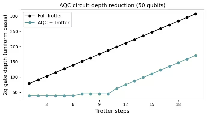
Step 2c — one-layer ansatz: 2971 parameters, 2q depth (uniform basis) = 39
Step 2c — two-layer ansatz: 3412 parameters, 2q depth (uniform basis) = 45
  k=1: fidelity = 1.0000, 2q depth (uniform basis) = 39, 215.6s
  k=2: fidelity = 0.9676, 2q depth (uniform basis) = 39, 269.8s
  k=3: fidelity = 0.9014, 2q depth (uniform basis) = 39, 293.5s
  k=4: fidelity = 0.8755, 2q depth (uniform basis) = 39, 279.6s
  k=5: fidelity = 0.8450, 2q depth (uniform basis) = 39, 266.4s
  k=6: fidelity = 0.8146, 2q depth (uniform basis) = 39, 371.0s

E0626 02:59:07.229070 1508496 slow_operation_alarm.cc:73] 
********************************
[Compiling module jit_MakeArrayFn for CPU] Very slow compile? If you want to file a bug, run with envvar XLA_FLAGS=--xla_dump_to=/tmp/foo and attach the results.
********************************
E0626 02:59:21.713796 1508477 slow_operation_alarm.cc:140] The operation took 2m14.484932074s

********************************
[Compiling module jit_MakeArrayFn for CPU] Very slow compile? If you want to file a bug, run with envvar XLA_FLAGS=--xla_dump_to=/tmp/foo and attach the results.
********************************

k=7: fidelity = 0.7312, 2q depth (uniform basis) = 45, 10865.3s
  k=8: fidelity = 0.7720, 2q depth (uniform basis) = 45, 1450.3s
  k=9: fidelity = 0.7316, 2q depth (uniform basis) = 45, 3388.6s

E0626 07:21:05.148724 1508496 slow_operation_alarm.cc:73] 
********************************
[Compiling module jit_MakeArrayFn for CPU] Very slow compile? If you want to file a bug, run with envvar XLA_FLAGS=--xla_dump_to=/tmp/foo and attach the results.
********************************
E0626 07:21:24.286095 1508477 slow_operation_alarm.cc:140] The operation took 2m19.137566498s

********************************
[Compiling module jit_MakeArrayFn for CPU] Very slow compile? If you want to file a bug, run with envvar XLA_FLAGS=--xla_dump_to=/tmp/foo and attach the results.
********************************

k=10: fidelity = 0.6726, 2q depth (uniform basis) = 45, 3396.1s

Step 2d — assembled 20 circuits
  At step 20 (uniform basis): Trotter 2q depth = 307, AQC+Trotter 2q depth = 171; 2q gates: Trotter = 3775, AQC+Trotter = 1913

Output of the previous code cell

Backend: ibm_fez
Transpiled 2q depth (deepest, ISA on ibm_fez): 105 (2q gates: 2574)
Job ID: d8v39vhropqc738biotg

Output of the previous code cell

تُعيد النتائج العتادية إنتاج السمات الرئيسية لمتصل اثنين-سبينون: تتركز شدة التشتت بالقرب من متجه الموجة المضاد للمغناطيسية $q = \pi$ عند طاقة منخفضة وتكون محدودة من الأسفل بتشتت السبينون الجيبي، مع متصل واسع من الوزن الطيفي فوقه بدلاً من نمط واحد حاد. هذا هو نفس التركيب المقاس بتشتت النيوترونات غير المرن على KCuF $_3$ ، ويتحقق من سير العمل الكامل لتحضير الحالة الأرضية، والاضطراب، وتطور تروتر المضغوط بـ AQC، والقياس المخفف الأخطاء على مقياس 50 كيوبتاً.

الخطوات التالية

إذا وجدت هذا العمل مثيراً للاهتمام، فقد تهتم بالمواد التالية:

توصيات

محاكاة تشتت النيوترونات بسير عمل Serverless لديناميكيات AQC + تروتر — دليل تعليمي مرافق يُشغّل نفس هذه التجربة عبر قالب دالة منشور في Qiskit Serverless
Lee et al.، "قياس محاكاة الكم مرجعياً بتجارب تشتت النيوترونات" (arXiv:2603.15608) — الورقة البحثية المرجعية التي يستند إليها هذا الدليل التعليمي
تقنيات تخفيف وقمع الأخطاء — DD وتمويه باولي وTREX المستخدمة في التجارب العتادية
التجميع الكمومي التقريبي لدوائر التطور الزمني — دليل تعليمي عن AQC-Tensor
توثيق AQC-Tensor

مخرجات التعلم​

المتطلبات المسبقة​

الخلفية​

تشتت النيوترونات غير المرن وعامل البنية الديناميكي​

KCuF3_33​: مغناطيس نموذجي من نوع سائل لوتينجر​

ماذا نُحاكي ونقيس​

سير عمل محاكاة الكم​

التجميع الكمومي التقريبي (AQC)​

محاكاة MPS​

المتطلبات​

الإعداد​

مثال محاكي صغير المقياس​

الخطوة 1: تعيين المدخلات الكلاسيكية إلى مسألة كمومية​

الخطوة 2: تحسين المسألة لتنفيذها على العتاد الكمومي​

الخطوة 3: التنفيذ باستخدام أوليات Qiskit​

الخطوة 4: معالجة النتيجة بعد الحصول عليها وإعادتها بالشكل الكلاسيكي المطلوب​

التنفيذ العتادي واسع النطاق​

الخطوات التالية​

مخرجات التعلم

المتطلبات المسبقة

الخلفية

تشتت النيوترونات غير المرن وعامل البنية الديناميكي

KCuF $_3$ : مغناطيس نموذجي من نوع سائل لوتينجر

ماذا نُحاكي ونقيس

سير عمل محاكاة الكم

التجميع الكمومي التقريبي (AQC)

محاكاة MPS

المتطلبات

الإعداد

مثال محاكي صغير المقياس

الخطوة 1: تعيين المدخلات الكلاسيكية إلى مسألة كمومية

الخطوة 2: تحسين المسألة لتنفيذها على العتاد الكمومي

الخطوة 3: التنفيذ باستخدام أوليات Qiskit

الخطوة 4: معالجة النتيجة بعد الحصول عليها وإعادتها بالشكل الكلاسيكي المطلوب

التنفيذ العتادي واسع النطاق

الخطوات التالية