بدء دافئ لـ QAOA باستخدام إضافة Qiskit لمخطط التحسين (Optimization Mapper)

تقدير الاستخدام: 9 دقائق على معالج Heron r3 (ملاحظة: هذا تقدير فقط. قد يختلف وقت التشغيل الفعلي لديك.)

مخرجات التعلم

• كيفية تعيين مسألة قطع أعظمي إلى صياغة تحسين ثنائي تربيعي غير مقيد (QUBO) باستخدام qiskit-addon-opt-mapper

• كيفية تنفيذ وتشغيل QAOA القياسي على محاكي

• كيفية تطبيق WS-QAOA بحساب تخفيف البرنامج التربيعي (QP) وبناء دارة البدء الدافئ

• كيفية مقارنة تقارب الطاقة وجودة الحل بين QAOA القياسي وWS-QAOA

المتطلبات المسبقة

• البرنامج التعليمي لـ QAOA

• البرنامج التعليمي المتقدم لـ QAOA

الخلفية

خوارزمية التحسين التقريبي الكمومي (QAOA) هي خوارزمية هجينة كمومية-كلاسيكية مصممة لحل مسائل التحسين التوافقي مثل القطع الأعظمي وصياغات QUBO العامة. للاطلاع على مقدمة أساسية لـ QAOA في Qiskit، راجع البرنامج التعليمي لـ QAOA؛ لتقنيات بناء دارات أكثر تقدماً، راجع البرنامج التعليمي المتقدم لـ QAOA.

في QAOA القياسي:

• الحالة الابتدائية هي التراكب المنتظم $|+\rangle^{\otimes n}$.
• تُهيَّأ المعاملات المتغيرة بشكل عشوائي.
• يبحث محسِّن كلاسيكي عن المعاملات التي تُقلل دالة التكلفة.

مع ذلك، بالنسبة لأحجام المسائل العملية والعتاد الكمومي المشوش، يمكن أن تؤدي التهيئة العشوائية إلى تقارب بطيء، وقيم صغرى محلية سيئة، وزيادة تكلفة التحسين.

QAOA بالبدء الدافئ (WS-QAOA) يحسّن ذلك بدمج رؤى التحسين الكلاسيكية مباشرة في الدارة الكمومية. يتّبع هذا البرنامج التعليمي الطرائق التي قدّمها إيغر ومارتشيك وويرنر في Warm-starting quantum optimization. الفكرة الرئيسية هي:

1. حل تخفيف متصل للمسألة الثنائية الأصلية (برنامج تربيعي على $[0,1]^n$ بدلاً من $\{0,1\}^n$).

2. ترميز الحل المُخفَّف $c^*_i \in [0,1]$ في حالة ابتدائية مخصصة باستخدام زوايا دوران $Y$، $\theta_i = 2\arcsin(\sqrt{c^*_i})$، بحيث يبدأ الكيوبت $i$ في حالة يكون فيها احتمال قياس $|1\rangle$ هو $c^*_i$.

3. استبدال خالط $X$ القياسي بخالط مخصص تكون حالته الأرضية هي حالة البدء الدافئ الابتدائية، مما يضمن أن الخوارزمية تبدأ قريباً من الحل الكلاسيكي ويمكنها استكشاف الجوار.

يقصّ معامل تنظيم $\varepsilon \in [0, 0.5]$ قيمة $c^*_i$ بعيداً عن 0 و1 لتجنب مشاكل الوصولية؛ لا يمكن تحريك الكيوبتات المُهيّأة في $|0\rangle$ أو $|1\rangle$ بواسطة هاميلتوني التكلفة. عند $\varepsilon = 0.5$، يختزل WS-QAOA بالضبط إلى QAOA القياسي.

تستخدم نمذجة المسألة حزمة qiskit-addon-opt-mapper، التي تبني فئة التطبيق Maxcut فيها QUBO مباشرة من رسم بياني، وتُعيّن محوّلاتها ومترجماتها المسألة الناتجة إلى هاميلتونيات كمومية.

المتطلبات

قبل بدء هذا البرنامج التعليمي، تأكد من تثبيت ما يلي:

• حزمة تطوير Qiskit SDK الإصدار 2.0 أو أحدث، مع دعم التصور

• Qiskit Runtime الإصدار 0.43 أو أحدث (pip install qiskit-ibm-runtime)

• إضافة Qiskit لمخطط التحسين (Optimization Mapper) (pip install qiskit-addon-opt-mapper)

• SciPy (pip install scipy)

• NetworkX (pip install networkx)

الإعداد

استورد جميع المكتبات المطلوبة وعرّف الدوال المساعدة المستخدمة طوال هذا البرنامج التعليمي.

# Added by doQumentation — required packages for this notebook
!pip install -q matplotlib networkx numpy qiskit qiskit-addon-opt-mapper qiskit-ibm-runtime scipy

import numpy as np
import matplotlib.pyplot as plt
import networkx as nx
from scipy.optimize import minimize

from qiskit.circuit import QuantumCircuit, ParameterVector
from qiskit.circuit.library import qaoa_ansatz
from qiskit.quantum_info import Statevector
from qiskit.primitives import StatevectorEstimator, StatevectorSampler
from qiskit.transpiler.preset_passmanagers import generate_preset_pass_manager
from qiskit_ibm_runtime import (
    QiskitRuntimeService,
    Session,
    EstimatorOptions,
    EstimatorV2 as Estimator,
    SamplerV2 as Sampler,
)

from qiskit_addon_opt_mapper.applications import Maxcut
from qiskit_addon_opt_mapper.converters import OptimizationProblemToQubo
from qiskit_addon_opt_mapper.translators import to_ising

مثال محاكي صغير النطاق

نستخدم مسألة قطع أعظمي صغيرة على رسم بياني موزون كمثال تشغيلي. يسأل القطع الأعظمي: بالنظر إلى رسم بياني $G=(V,E)$ بأوزان حواف $w_{ij}$، أوجد تقسيماً للرؤوس إلى مجموعتين $S$ و$\bar{S}$ يُعظّم الوزن الكلي للحواف العابرة للقطع.

كمسألة تقليل QUBO، يمكن كتابة القطع الأعظمي كالتالي: $\min_{x \in \{0,1\}^n} -\sum_{(i,j) \in E} w_{ij}(x_i + x_j - 2x_i x_j)$

نعمل مع رسم بياني بأربع عُقد لجعله قابلاً للتعامل على محاكي.

الخطوة 1: تعيين المدخلات الكلاسيكية إلى مسألة كمومية

نعرّف مسألة القطع الأعظمي باستخدام فئة التطبيق Maxcut من qiskit-addon-opt-mapper، التي تبني صياغة QUBO مباشرة من رسم بياني. ثم نحوّلها إلى QUBO ونترجمها إلى هاميلتوني إيزنغ (SparsePauliOp) مناسب لـ QAOA. كما نحل التخفيف المتصل لـ QUBO — باستبدال القيد الثنائي $x_i \in \{0,1\}$ بـ $x_i \in [0,1]$ — للحصول على نقطة البدء الدافئ الابتدائية $c^*$.

# Define a 4-node weighted graph for the max-cut problem
n_nodes = 4
edges = [(0, 1, 1.0), (0, 2, 1.0), (1, 2, 1.0), (1, 3, 1.0), (2, 3, 1.0)]

G = nx.Graph()
G.add_nodes_from(range(n_nodes))
G.add_weighted_edges_from(edges)

pos = nx.spring_layout(G, seed=42)
edge_labels = {(u, v): d["weight"] for u, v, d in G.edges(data=True)}

fig, ax = plt.subplots(figsize=(4, 3))
nx.draw(G, pos, with_labels=True, node_color="lightblue", ax=ax)
nx.draw_networkx_edge_labels(G, pos, edge_labels=edge_labels, ax=ax)
ax.set_title("Max-Cut graph")
plt.tight_layout()
plt.show()

يحتوي الرسم البياني على خمس حواف. يُقسّم القطع الأعظمي الأمثل العُقد إلى $S = \{0, 3\}$ و$\bar{S} = \{1, 2\}$ (أو مكمّله)، مما يقطع أربعاً من الحواف الخمس بقيمة قطع 4.

# Build the max-cut problem directly from the NetworkX graph using the
# Maxcut application class. Internally it constructs the QUBO
#   minimize  -sum_{(i,j) in E} w_ij * (x_i + x_j - 2*x_i*x_j)
# (each edge contributes -w to the linear terms and +2w to the quadratic
# term), so we get the same OptimizationProblem without the boilerplate.
maxcut = Maxcut(G)
prob = maxcut.to_optimization_problem()
print(prob.prettyprint())

Problem name: Max-cut

Maximize
  -2*x_0*x_1 - 2*x_0*x_2 - 2*x_1*x_2 - 2*x_1*x_3 - 2*x_2*x_3 + 2*x_0 + 3*x_1
  + 3*x_2 + 2*x_3

Subject to
  No constraints

  Binary variables (4)
    x_0 x_1 x_2 x_3

تُغلّف الفئة Maxcut بناء QUBO حتى لا نضطر إلى توسيع هدف القطع الأعظمي يدوياً. يُظهر الهدف المطبوع معامل كل متغير الخطي (مقدار مساهمته الفردية في القطع) والمعامل التربيعي لكل حد متقاطع (العقوبة على وضع عقدتين متجاورتين على نفس الجانب). يدعم كائن OptimizationProblem الأساسي الذي تُرجعه to_optimization_problem() المتغيرات الثنائية والصحيحة والمتصلة والسبينية، وهو نفس الكائن الذي تتوقعه المحوّلات والمترجمات المستخدمة في الخطوة التالية.

# Convert the OptimizationProblem to a QUBO, then translate to an Ising Hamiltonian
#
# The substitution x_i = (1 - z_i)/2  maps binary variables to spin operators,
# yielding a Hamiltonian H_C = sum_i h_i Z_i + sum_{i<j} J_ij Z_i Z_j + constant.
# QAOA minimizes <H_C> to find the ground state, which encodes the optimal cut.
converter = OptimizationProblemToQubo()
qubo = converter.convert(prob)

cost_operator, offset = to_ising(qubo)
n_qubits = cost_operator.num_qubits

print(f"Cost Hamiltonian H_C ({n_qubits} qubits):")
print(cost_operator)
print(f"\nOffset (constant shift): {offset}")
print("  QUBO value = Ising energy + offset")

Cost Hamiltonian H_C (4 qubits):
SparsePauliOp(['IIZZ', 'IZIZ', 'IZZI', 'ZIZI', 'ZZII'],
              coeffs=[0.5+0.j, 0.5+0.j, 0.5+0.j, 0.5+0.j, 0.5+0.j])

Offset (constant shift): -2.5
  QUBO value = Ising energy + offset

يُعيد المترجم to_ising كائن SparsePauliOp يمثل $H_C$ وقيمة عددية offset بحيث $\text{QUBO value} = \langle H_C \rangle + \text{offset}$. لمسألة القطع الأقصى هذه بأوزان واحدية جميعها، $h_i = 0$ لجميع الكيوبتات (الرسم البياني متماثل في الحدود الخطية بعد التعويض $x_i \to z_i$)، وتُسهم كل حافة باقتران $Z_i Z_j$ بقوة $+0.5$. تقابل القيمة الذاتية الدنيا لـ $H_C$ القطع الأقصى.

# Solve the continuous (QP) relaxation to obtain the warm-start point c*
#
# The QP relaxation replaces the binary constraint x_i in {0,1} with x_i in [0,1]
# and minimizes the same quadratic objective. Its solution c*_i gives the
# probability that variable i should be 1 according to the classical relaxation.
#
# The max-cut QUBO has a non-convex quadratic matrix (negative eigenvalues),
# so the relaxed problem has multiple local minima. A naive single start from
# [0.5,...,0.5] converges to the symmetric saddle point c* = [0.5,...,0.5],
# which carries no useful structural information about the problem.
# Multi-start optimization is used to reliably find the global minimum.
Q = qubo.objective.quadratic.to_array(symmetric=True)
mu = qubo.objective.linear.to_array()

def qp_objective(x_cont):
    """Continuous relaxation of the QUBO objective."""
    return x_cont @ Q @ x_cont + mu @ x_cont + qubo.objective.constant

bounds = [(0.0, 1.0)] * n_qubits

rng = np.random.default_rng(42)
best_val = np.inf
c_star = None
for _ in range(200):
    x0 = rng.uniform(0.0, 1.0, n_qubits)
    result = minimize(qp_objective, x0, method="L-BFGS-B", bounds=bounds)
    if result.fun < best_val:
        best_val = result.fun
        c_star = result.x

print(f"QP relaxation solution c* = {np.round(c_star, 4)}")
print(f"QP objective value        = {best_val:.4f}")

QP relaxation solution c* = [1. 0. 0. 1.]
QP objective value        = -4.0000

يجد المحلّل متعدد البدايات $c^* = [1, 0, 0, 1]$ (أو مكمّله $[0, 1, 1, 0]$)، وهو الحل الثنائي الأمثل الفعلي. بالنسبة لهذه المسألة يكون تخفيف QP محكماً، إذ يتطابق الحد الأدنى المتصل مع الأمثل الصحيح، مما يعني أن التخفيف يحدد فوراً أفضل قطع. بعد التنظيم بـ $\varepsilon = 0.25$ في الخطوة 2، سيُرمّز هذا الحل في حالة البدء الدافئ الابتدائية.

الخطوة 2: تحسين المسألة لتنفيذ العتاد الكمومي

نبني دارتَي QAOA ونُحضّر زوايا البدء الدافئ من حل QP.

يستخدم QAOA القياسي التراكب المنتظم $|+\rangle^{\otimes n}$ كحالة ابتدائية وخالط $X$ القياسي $H_M = -\sum_i X_i$، المُنفَّذ كـ $\prod_i R_X(-2\beta)$ لكل طبقة.

QAOA بالبدء الدافئ (WS-QAOA) من [1] يُجري تغييرين بنيويين لكل كيوبت $i$:

• الحالة الابتدائية: $R_Y(\theta_i)|0\rangle$ مع $\theta_i = 2\arcsin(\sqrt{c^*_i})$، بحيث يساوي احتمال قياس $|1\rangle$ القيمة $c^*_i$.
• الخالط المخصص: $R_Y(\theta_i)\, R_Z(-2\beta)\, R_Y(-\theta_i)$، الذي له $R_Y(\theta_i)|0\rangle$ كحالة أرضية. هذا يعني أن WS-QAOA يبدأ في الحالة الأرضية لخالطه الخاص، نفس الخاصية التي يحققها QAOA القياسي مع $|+\rangle$ وخالط $X$.

ملاحظة حول الطبقات: عند p=1 (طبقة QAOA واحدة)، يقتصر QAOA القياسي تحليلياً على حوالي 49% من الطاقة المثلى على الرسوم البيانية التي تحتوي على مثلثات (يحتوي هذا الرسم البياني على المثلث 0-1-2). يتجاوز البدء الدافئ هذا القيد بترميز معرفة مسبقة عن الحل مباشرة في الحالة الابتدائية.

# Number of QAOA layers (each layer = one cost unitary + one mixer unitary)
p = 1

# Regularization: clip c* to [epsilon, 1-epsilon] so no qubit is initialized
# in |0> or |1>, which would freeze it under the cost Hamiltonian.
epsilon = 0.25

c_clipped = np.clip(c_star, epsilon, 1 - epsilon)
thetas = 2 * np.arcsin(np.sqrt(c_clipped))

print(f"Continuous relaxation c*  = {np.round(c_star, 4)}")
print(f"After regularization      = {np.round(c_clipped, 4)}")
print(f"Warm-start angles theta   = {np.round(thetas, 4)} radians")
print()
print("Angle interpretation:")
print("  theta = 0      <->  c* = 0   (qubit points toward |0>)")
print(
    "  theta = pi/2   <->  c* = 0.5 (qubit in equal superposition, like |+>)"
)
print("  theta = pi     <->  c* = 1   (qubit points toward |1>)")

Continuous relaxation c*  = [1. 0. 0. 1.]
After regularization      = [0.75 0.25 0.25 0.75]
Warm-start angles theta   = [2.0944 1.0472 1.0472 2.0944] radians

Angle interpretation:
  theta = 0      <->  c* = 0   (qubit points toward |0>)
  theta = pi/2   <->  c* = 0.5 (qubit in equal superposition, like |+>)
  theta = pi     <->  c* = 1   (qubit points toward |1>)

بعد القص، تصبح $c^* = 1$ هي $1 - \varepsilon = 0.75$ وتصبح $c^* = 0$ هي $\varepsilon = 0.25$. الزوايا الناتجة $\theta \approx [2.09, 1.05, 1.05, 2.09]$ راديان تُدوّر الكيوبتات 0 و3 بقوة نحو $|1\rangle$ والكيوبتات 1 و2 نحو $|0\rangle$، مما يُرمّز مباشرة بنية القطع الأمثل في الحالة الكمومية الابتدائية.

def apply_cost_unitary(qc, cost_op, gamma):
    """Apply exp(-i * gamma * H_C) to the circuit.

    Each Pauli term in H_C contributes a rotation gate:
      - Single-Z term h_i * Z_i  ->  RZ(2 * gamma * h_i) on qubit i
      - Two-Z term J_ij * Z_i Z_j  ->  CNOT, RZ(2 * gamma * J_ij), CNOT
    """
    for pauli_term, coeff in zip(cost_op.paulis, cost_op.coeffs):
        indices = [
            j for j, q in enumerate(pauli_term.to_label()[::-1]) if q == "Z"
        ]
        if len(indices) == 1:
            qc.rz(2 * gamma * coeff.real, indices[0])
        elif len(indices) == 2:
            qc.cx(indices[0], indices[1])
            qc.rz(2 * gamma * coeff.real, indices[1])
            qc.cx(indices[0], indices[1])

def build_ws_qaoa(cost_op, n_layers, n_qubits, thetas):
    """WS-QAOA: warm-start initial state + custom per-qubit mixer.

    Per Egger et al. (2021) Eq. (1)-(2):
      Initial state per qubit i:  R_Y(theta_i) |0>
      Mixer gate per qubit i:     R_Y(theta_i) R_Z(-2*beta) R_Y(-theta_i)
    """
    gammas = ParameterVector("γ", n_layers)
    betas = ParameterVector("β", n_layers)
    qc = QuantumCircuit(n_qubits)
    for i, theta in enumerate(thetas):
        qc.ry(theta, i)  # warm-start initial state
    for k in range(n_layers):
        apply_cost_unitary(qc, cost_op, gammas[k])
        for i, theta in enumerate(thetas):
            qc.ry(theta, i)
            qc.rz(-2 * betas[k], i)
            qc.ry(-theta, i)
    return qc, gammas, betas

# Standard QAOA via the Qiskit built-in helper:
# qaoa_ansatz prepares |+>^n, then alternates exp(-i*gamma*H_C) with the
# default X-mixer for `reps` layers. The returned circuit exposes the
# variational parameters via std_qc.parameters.
std_qc = qaoa_ansatz(cost_operator, reps=p)

# WS-QAOA: keep the custom builder. The per-qubit mixer
# R_Y(theta_i) R_Z(-2*beta) R_Y(-theta_i) is implemented as an explicit gate
# sequence rather than as a SparsePauliOp, so we construct the circuit
# directly to stay close to the Egger et al. (2021) formulation.
ws_qc, ws_gammas, ws_betas = build_ws_qaoa(cost_operator, p, n_qubits, thetas)

بالنسبة للمخطط القياسي نُفوّض إلى qaoa_ansatz، التي تُنشئ $|+\rangle^{\otimes n}$، وتُطبق وحدوية التكلفة، وتُطبق خالط $X$ الافتراضي لكل طبقة من طبقات reps. بالنسبة لـ WS-QAOA نحتفظ بالمساعد الصريح build_ws_qaoa لأن الخالط لكل كيوبت $R_Y(\theta)\,R_Z(-2\beta)\,R_Y(-\theta)$ يُعبَّر عنه كتسلسل بوابات وليس كمجموع من مؤثرات باولي. يقرأ المساعد apply_cost_unitary مباشرة من هاميلتوني SparsePauliOp، لذا فهو يتعامل مع أي مسألة QUBO دون بناء دارة يدوي.

print("Standard QAOA circuit (p=1):")
std_qc.draw("mpl", fold=-1)

Standard QAOA circuit (p=1):

print("\nWS-QAOA circuit (p=1):")
ws_qc.draw("mpl", fold=-1)

WS-QAOA circuit (p=1):

تتّبع كلتا الدارتين نفس البنية: طبقة تحضير حالة ابتدائية، ثم $p$ طبقات متناوبة من وحدوية التكلفة ووحدوية الخالط. في دارة WS-QAOA، تُرمّز بوابات $R_Y$ الافتتاحية $c^*$، ويستبدل الخالط كل $R_X$ بثلاثية $R_Y$–$R_Z$–$R_Y$ مقترنة. ينمو فرق عمق الدارة بين الاثنتين خطياً مع $p$، لكنه يبقى قابلاً للإدارة عند عمق منخفض.

الخطوة 3: التنفيذ باستخدام بدائيات Qiskit

نستخدم StatevectorEstimator لمحاكاة دقيقة خالية من الضجيج. تُشغّل الدالة minimize من SciPy مع محسّن COBYLA الحلقة المتغيرة، مستدعيةً المُقدِّر عند كل تكرار لتقييم $\langle H_C \rangle$ لمجموعة معاملات معطاة $(\gamma, \beta)$.

تستخدم الخوارزميتان معاملات ابتدائية مختلفة تعكس ما يعرفه كل منهما قبل التحسين:

• QAOA القياسي: تهيئة عشوائية في $[0, \pi]$ — مناسبة لأنه لا تتوفر معلومات بنيوية.
• WS-QAOA: $\gamma = 0$، $\beta = \pi/4$ — عند $\gamma=0$ تكون وحدوية التكلفة هي المطابقة، لذا يأخذ أول تقييم للدارة عينة مباشرة من حالة البدء الدافئ الابتدائية. هذا يعطي COBYLA إشارة بداية قوية متوافقة مع الحل الكلاسيكي.

estimator = StatevectorEstimator()

def make_cost_fn(circuit, param_order, cost_op, estimator, history):
    """Return a scalar cost function compatible with scipy.optimize.minimize."""

    def cost_fn(params):
        bound = circuit.assign_parameters(dict(zip(param_order, params)))
        job = estimator.run([(bound, cost_op)])
        energy = job.result()[0].data.evs.real
        history.append(energy)
        return energy

    return cost_fn

# Standard QAOA: random initialization
np.random.seed(42)
std_param_order = list(std_qc.parameters)
std_params0 = np.random.uniform(0, np.pi, len(std_param_order))
std_history = []

std_result = minimize(
    make_cost_fn(
        std_qc, std_param_order, cost_operator, estimator, std_history
    ),
    std_params0,
    method="COBYLA",
    options={"maxiter": 300, "rhobeg": 0.5},
)
print(f"Standard QAOA optimal energy : {std_result.fun:.4f}")
print(f"  optimal params: {std_result.x.round(4)}")
print(f"  optimizer calls: {len(std_history)}")

# WS-QAOA: informed initialization
ws_params0 = np.concatenate([np.zeros(p), np.full(p, np.pi / 4)])
ws_history = []
ws_param_order = list(ws_gammas) + list(ws_betas)

ws_result = minimize(
    make_cost_fn(ws_qc, ws_param_order, cost_operator, estimator, ws_history),
    ws_params0,
    method="COBYLA",
    options={"maxiter": 300, "rhobeg": 0.5},
)
print(f"\nWS-QAOA optimal energy       : {ws_result.fun:.4f}")
print(
    f"  optimal params: gamma={ws_result.x[:p].round(4)}, beta={ws_result.x[p:].round(4)}"
)
print(f"  optimizer calls: {len(ws_history)}")

Standard QAOA optimal energy : -0.5859
  optimal params: [0.6803 2.0533]
  optimizer calls: 47

WS-QAOA optimal energy       : -1.5000
  optimal params: gamma=[-0.0001], beta=[1.5708]
  optimizer calls: 42

تعني نقطة بداية WS-QAOA المستنيرة أن COBYLA يبدأ بقيمة طاقة ذات معنى قريبة من حل البدء الدافئ، بينما يبدأ QAOA القياسي من نقطة عشوائية أساساً على مشهد الطاقة. هذا الفرق في جودة البداية هو المحرك الرئيسي لفجوة التقارب الظاهرة في الخطوة 4.

# Compute the exact optimal energy by brute-force over all 2^n bitstrings
all_energies = [
    Statevector.from_label(format(k, f"0{n_qubits}b"))
    .expectation_value(cost_operator)
    .real
    for k in range(2**n_qubits)
]
optimal_energy = min(all_energies)

print(f"Exact optimal energy         : {optimal_energy:.4f}")
print(f"Standard QAOA approx. ratio  : {std_result.fun / optimal_energy:.4f}")
print(f"WS-QAOA approx. ratio        : {ws_result.fun / optimal_energy:.4f}")

Exact optimal energy         : -1.5000
Standard QAOA approx. ratio  : 0.3906
WS-QAOA approx. ratio        : 1.0000

تُعرَّف نسبة التقريب بأنها $\langle H_C \rangle_{\text{QAOA}} / E_{\text{opt}}$. بالنسبة لمسائل التقليل حيث $E_{\text{opt}} < 0$، تعني النسبة الأقرب إلى 1 أن الخوارزمية وجدت طاقة أقل (حلاً أفضل). البحث الشامل (brute-force) عبر جميع الحالات الأساسية $2^n$ ممكن فقط بالنسبة لـ $n$ صغير ويُستخدم كمرجع للحقيقة الأرضية.

الخطوة 4: المعالجة اللاحقة وإرجاع النتيجة بالتنسيق الكلاسيكي المطلوب

نُصوّر التقارب، ونأخذ عينة من الدارات المُحسَّنة للحصول على حلول سلاسل بتات، ونفكّ ترميز سلاسل البتات تلك إلى تقسيمات قطع أعظمي، ونلخّص النتائج النهائية.

fig, ax = plt.subplots(figsize=(7, 4))
ax.plot(std_history, label="Standard QAOA", alpha=0.85)
ax.plot(ws_history, label="WS-QAOA", alpha=0.85)
ax.axhline(
    optimal_energy,
    color="k",
    linestyle="--",
    label=f"Exact optimal ({optimal_energy:.2f})",
)
ax.set_xlabel("Optimizer call")
ax.set_ylabel(r"$\langle H_C \rangle$")
ax.set_title("Convergence: Standard QAOA vs. WS-QAOA")
ax.legend()
plt.tight_layout()
plt.show()

يُظهر مخطط التقارب الطاقة $\langle H_C \rangle$ عند كل تقييم لدالة COBYLA. يقتصر QAOA القياسي عند $p=1$ على حوالي 49% من الطاقة المثلى على هذا الرسم البياني (الحد الأقصى النظري لـ QAOA بـ $p=1$ على الرسوم البيانية ذات المثلثات)، مستقراً حول $-0.74$. أما WS-QAOA، المُهيَّأ قريباً من الحل الأمثل، فيتقارب بسرعة إلى ما يقرب من $-1.50$ (الأمثل بالضبط) بعدد أقل بكثير من التكرارات. هذا يُظهر الميزة الرئيسية للبدء الدافئ: عند نفس عمق الدارة، يصل إلى حل أفضل بكثير.

# Sample the optimized circuits to recover the most probable bitstring solutions
sampler = StatevectorSampler()
shots = 1024

def get_best_bitstring(circuit, param_order, optimal_params, sampler, shots):
    bound = circuit.assign_parameters(dict(zip(param_order, optimal_params)))
    bound.measure_all()
    job = sampler.run([bound], shots=shots)
    counts = job.result()[0].data.meas.get_counts()
    return max(counts, key=counts.get), counts

def evaluate_cut(bitstring, G):
    """Compute the Max-Cut value for a bitstring node assignment."""
    x = [int(b) for b in bitstring]
    cut_val = sum(
        w for u, v, w in G.edges.data("weight", default=1) if x[u] != x[v]
    )
    set0 = [i for i, b in enumerate(bitstring) if b == "0"]
    set1 = [i for i, b in enumerate(bitstring) if b == "1"]
    return cut_val, set0, set1

# Qiskit bitstring ordering: rightmost character = qubit 0
def decode_bitstring(bs):
    return bs[::-1]

std_best, std_counts = get_best_bitstring(
    std_qc, std_param_order, std_result.x, sampler, shots
)
ws_best, ws_counts = get_best_bitstring(
    ws_qc, ws_param_order, ws_result.x, sampler, shots
)

std_cut, std_s0, std_s1 = evaluate_cut(decode_bitstring(std_best), G)
ws_cut, ws_s0, ws_s1 = evaluate_cut(decode_bitstring(ws_best), G)

print(f"Standard QAOA most-probable bitstring : {std_best}")
print(f"  Partition: S={std_s0}, S̄={std_s1}  |  cut value = {std_cut}")
print()
print(f"WS-QAOA most-probable bitstring       : {ws_best}")
print(f"  Partition: S={ws_s0}, S̄={ws_s1}  |  cut value = {ws_cut}")

Standard QAOA most-probable bitstring : 0110
  Partition: S=[0, 3], S̄=[1, 2]  |  cut value = 4.0

WS-QAOA most-probable bitstring       : 0110
  Partition: S=[0, 3], S̄=[1, 2]  |  cut value = 4.0

تُرجَع سلاسل البتات من Sampler مع الكيوبت 0 في أقصى اليمين، لذا فإن عكس السلسلة يُعيّن الفهرس $i$ إلى المتغير $x_i$. قيمة القطع هي الوزن الكلي للحواف التي تعبر التقسيم، وهو ما تهدف مسألة القطع الأعظمي إلى تعظيمه. قيمة قطع تساوي 4 تستخدم أربعاً من الحواف الخمس المتاحة، وهو الحد الأقصى النظري لهذا الرسم البياني.

# Visualize the WS-QAOA solution on the graph
fig, axes = plt.subplots(1, 2, figsize=(8, 3))

for ax, s0, s1, cut, title in [
    (axes[0], std_s0, std_s1, std_cut, f"Standard QAOA (cut = {std_cut})"),
    (axes[1], ws_s0, ws_s1, ws_cut, f"WS-QAOA (cut = {ws_cut})"),
]:
    colors = ["skyblue" if i in s0 else "salmon" for i in G.nodes()]
    nx.draw(G, pos, with_labels=True, node_color=colors, ax=ax)
    nx.draw_networkx_edge_labels(G, pos, edge_labels=edge_labels, ax=ax)
    ax.set_title(title)

plt.tight_layout()
plt.show()

# Summary
# to_ising offset: QUBO value = Ising energy + offset, so Max-Cut value = -(Ising energy + offset)
optimal_cut = -(optimal_energy + offset)
print("=== Summary ===")
print(
    f"{'Method':<20} {'Ising energy':>14} {'Cut value':>12} {'Approx. ratio':>15}"
)
print("-" * 65)
print(
    f"{'Standard QAOA':<20} {std_result.fun:>14.4f} {std_cut:>12} {std_result.fun/optimal_energy:>15.4f}"
)
print(
    f"{'WS-QAOA':<20} {ws_result.fun:>14.4f} {ws_cut:>12} {ws_result.fun/optimal_energy:>15.4f}"
)
print(
    f"{'Exact optimal':<20} {optimal_energy:>14.4f} {optimal_cut:>12.0f} {'1.0000':>15}"
)

=== Summary ===
Method                 Ising energy    Cut value   Approx. ratio
-----------------------------------------------------------------
Standard QAOA               -0.5859          4.0          0.3906
WS-QAOA                     -1.5000          4.0          1.0000
Exact optimal               -1.5000            4          1.0000

يُلوّن تصور الرسم البياني كل عقدة حسب تعيين تقسيمها (أزرق = $S$، برتقالي = $\bar{S}$). الحواف التي تعبر التقسيم (تربط عُقداً مختلفة اللون) هي التي تُحتسب في القطع.

تجد كلتا الطريقتين سلسلة بتات بقيمة قطع 4، لكن لأسباب مختلفة جداً. من المهم ملاحظة أن مخطط التقارب وسلسلة البتات المأخوذة عينياً يقيسان أمرين مختلفين:

• يتتبع مخطط التقارب متوسط الطاقة $\langle H_C \rangle$ للحالة الكمومية الكاملة، وهو متوسط موزون عبر جميع سلاسل البتات في التراكب. يتقارب QAOA القياسي إلى حوالي $-0.62$، أعلى بكثير من الأمثل $-1.50$، مما يعني أن حالته الكمومية موزّعة عبر العديد من سلاسل البتات دون المثلى ولا تتضمن الإجابة الصحيحة إلا أحياناً.

• سلسلة البتات المأخوذة عينياً هي سحبة واحدة من تلك الحالة. حظي QAOA القياسي بالحظ هنا؛ صادف أن التقسيم الأمثل كان النتيجة الأكثر تكراراً حتى من حالة منتشرة. في مسائل أصعب، أو عتاد أكثر ضجيجاً، أو مع تنافس المزيد من الحلول المرشحة، ينفد هذا الحظ.

في المقابل، يتقارب WS-QAOA بمتوسط طاقته وصولاً إلى $-1.50$، مما يعني أن حالته الكمومية مُركَّزة على سلاسل البتات المثلى. تُرجع كل لقطة تقريباً الإجابة الصحيحة، لذا يُعثر على الحل بشكل موثوق بدلاً من الصدفة.

النتيجة العملية: على هذا المحاكي الصغير الخالي من الضجيج قد يبدو الفرق طفيفاً، لكن عند أحجام مسائل أكبر أو على عتاد حقيقي، تكون الحالة ذات متوسط طاقة قريب من الأمثل أكثر متانة بكثير من حالة تأخذ عينة الإجابة الصحيحة أحياناً فقط من توزيع منتشر.

# Compare the full probability distribution over cut values for both
# algorithms. The most-probable bitstring above only reveals the mode;
# this histogram exposes how much of the quantum state's probability mass
# lands on the optimal cut versus on suboptimal partitions.
def cut_value_distribution(counts, G, shots):
    dist = {}
    for bs, c in counts.items():
        cut, _, _ = evaluate_cut(decode_bitstring(bs), G)
        dist[cut] = dist.get(cut, 0.0) + c / shots
    return dist

std_cut_dist = cut_value_distribution(std_counts, G, shots)
ws_cut_dist = cut_value_distribution(ws_counts, G, shots)

cut_values = sorted(set(std_cut_dist) | set(ws_cut_dist))
std_probs = [std_cut_dist.get(c, 0.0) for c in cut_values]
ws_probs = [ws_cut_dist.get(c, 0.0) for c in cut_values]

fig, ax = plt.subplots(figsize=(7, 4))
x = np.arange(len(cut_values))
width = 0.4
ax.bar(
    x - width / 2, std_probs, width, label="Standard QAOA", color="steelblue"
)
ax.bar(x + width / 2, ws_probs, width, label="WS-QAOA", color="salmon")
ax.axvline(
    cut_values.index(optimal_cut),
    color="k",
    linestyle="--",
    alpha=0.4,
    label=f"Optimal cut = {optimal_cut:g}",
)
ax.set_xticks(x)
ax.set_xticklabels([f"{c:g}" for c in cut_values])
ax.set_xlabel("Cut value")
ax.set_ylabel("Probability")
ax.set_title(f"Probability of measuring each cut value ({shots} shots)")
ax.legend()
plt.tight_layout()
plt.show()

print(
    f"P(cut = {optimal_cut:g}) | Standard QAOA = "
    f"{std_cut_dist.get(optimal_cut, 0):.4f}  "
    f"WS-QAOA = {ws_cut_dist.get(optimal_cut, 0):.4f}"
)

P(cut = 4) | Standard QAOA = 0.4639  WS-QAOA = 1.0000

يُقيّم هذا المدرج التكراري ما اقترحه مخطط التقارب فقط. احتمال QAOA القياسي مُوزَّع عبر قيم قطع متعددة دون المثلى، لذا فإن فرصة أخذ عينة قطع أمثل قيمته أربعة في أي لقطة واحدة هي فقط جزء من الكتلة الكلية. يُركِّز WS-QAOA تقريباً كل احتماله على القطع الأمثل، لذا تُرجع كل لقطة تقريباً الإجابة الصحيحة. هذا هو التوقيع العملي لحالة تقارب متوسط طاقتها إلى طاقة الحالة الأرضية مقابل حالة صادف أنها تضمنت الحالة الأرضية في تراكب واسع.

مثال عتاد كبير النطاق

ضغط الخطوات 1-4 في كتلة كود واحدة

# Selecting a backend using real hardware
service = QiskitRuntimeService()
backend = service.least_busy(
    operational=True, simulator=False, min_num_qubits=127
)
print(f"Using backend: {backend.name}")

Using backend: ibm_boston

# ── Step 1a: Build the 40-node Max-Cut problem ─────────────────────────────
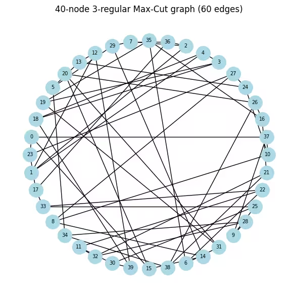
# A 3-regular graph (every node has exactly 3 neighbors) is a standard QAOA
N_LARGE = 40
G_large = nx.random_regular_graph(d=3, n=N_LARGE, seed=0)
edges_large = list(G_large.edges())
print(f"Graph: {N_LARGE} nodes, {len(edges_large)} edges (3-regular)")

# Visualize the graph so it is clear what problem we are solving before any
# quantum work. Nodes in a circular layout; each edge contributes +1 to the
# cut value when its endpoints land in different partitions.
pos_large = nx.circular_layout(G_large)
fig, ax = plt.subplots(figsize=(6, 6))
nx.draw(
    G_large,
    pos_large,
    with_labels=True,
    node_color="lightblue",
    node_size=400,
    font_size=7,
    ax=ax,
)
ax.set_title(f"40-node 3-regular Max-Cut graph ({len(edges_large)} edges)")
plt.tight_layout()
plt.show()

# Same Maxcut → OptimizationProblem → QUBO → Ising pipeline as the small example,
# applied to the 40-node graph.
prob_large = Maxcut(G_large).to_optimization_problem()
converter_large = OptimizationProblemToQubo()
qubo_large = converter_large.convert(prob_large)
cost_op_large, offset_large = to_ising(qubo_large)
n_qubits_large = cost_op_large.num_qubits
print(
    f"Cost operator: {n_qubits_large} qubits, {len(cost_op_large)} Pauli terms"
)

# ── Step 1b: QP relaxation (multi-start L-BFGS-B) ─────────────────────────
# Same multi-start approach as the small example. At 40 qubits the relaxed
# landscape has many more local minima, so 200 random starts are essential
# to find a low-energy warm-start point.
Q_large = qubo_large.objective.quadratic.to_array(symmetric=True)
mu_large = qubo_large.objective.linear.to_array()

def qp_obj_large(x):
    return x @ Q_large @ x + mu_large @ x + qubo_large.objective.constant

bounds_large = [(0.0, 1.0)] * n_qubits_large
rng_qp = np.random.default_rng(42)
best_val_large, c_star_large = np.inf, None

for _ in range(200):
    x0 = rng_qp.uniform(0.0, 1.0, n_qubits_large)
    res = minimize(qp_obj_large, x0, method="L-BFGS-B", bounds=bounds_large)
    if res.fun < best_val_large:
        best_val_large, c_star_large = res.fun, res.x

# Regularize and convert to rotation angles (same formula as small example)
epsilon_large = 0.25
c_clipped_large = np.clip(c_star_large, epsilon_large, 1 - epsilon_large)
thetas_large = 2 * np.arcsin(np.sqrt(c_clipped_large))
print(
    f"c* range: [{c_star_large.min():.3f}, {c_star_large.max():.3f}]  "
    f"theta range: [{thetas_large.min():.3f}, {thetas_large.max():.3f}] rad"
)

# Plot the distribution of c* values to see how much structure the relaxation
# extracted. Values near 0/1 mean confident assignments; values near 0.5 mean
# the classical solver was uncertain and quantum exploration is most needed there.
fig, ax = plt.subplots(figsize=(6, 3))
ax.hist(c_star_large, bins=20, color="steelblue", edgecolor="white")
ax.axvline(0.5, color="k", linestyle="--", label="Uniform prior (std QAOA)")
ax.set_xlabel(r"$c^*_i$")
ax.set_ylabel("Count")
ax.set_title(r"Distribution of warm-start values $c^*_i$ (40-node graph)")
ax.legend()
plt.tight_layout()
plt.show()

# ── Step 1c: Build WS-QAOA circuit ─────────────────────────────────────────
# Reuse build_ws_qaoa from the small-scale section unchanged; the helper
# scales automatically with n_qubits and the cost operator size.
p_large = 1
ws_qc_large, ws_gammas_large, ws_betas_large = build_ws_qaoa(
    cost_op_large, p_large, n_qubits_large, thetas_large
)
ws_qc_large.measure_all()

# ── Step 2: Transpile to hardware-native gates ──────────────────────────
# generate_preset_pass_manager compiles the abstract circuit to th
# gate set of the backend and inserts SWAP gates wherever the cost Hamiltonian
# couples qubits that are not directly connected on the processor.
pm = generate_preset_pass_manager(optimization_level=3, backend=backend)
ws_isa_large = pm.run(ws_qc_large)

ecr_count = ws_isa_large.count_ops().get("ecr", 0)
print(
    f"\nTranspiled circuit: 2Q depth={ws_isa_large.depth(lambda x: x.operation.num_qubits == 2)}"
)
ws_isa_large.draw("mpl", fold=-1)

Graph: 40 nodes, 60 edges (3-regular)

Cost operator: 40 qubits, 60 Pauli terms
c* range: [0.000, 1.000]  theta range: [1.047, 2.094] rad

Transpiled circuit: 2Q depth=86

# ── Classical baseline via simulated annealing ────────────────────
# Run SA before any hardware calls to get a strong classical reference cut
# value. SA is fast (seconds), needs no solver license, and reliably finds
# near-optimal solutions on 40-node graphs. We use sa_cut as the denominator
# for the approximation ratio instead of the looser QP upper bound.
#
# At each step we flip a random node and accept the move if it improves the
# cut, or with probability exp(delta/T) otherwise. Temperature T decays
# geometrically, allowing uphill moves early on to escape local minima.
def simulated_annealing_maxcut(
    G, seed=0, T0=2.0, T_min=1e-4, alpha=0.995, n_steps=100_000
):
    rng_sa = np.random.default_rng(seed)
    n = G.number_of_nodes()
    x = rng_sa.integers(0, 2, n)
    best_x = x.copy()
    best_cut = sum(1 for u, v in G.edges() if x[u] != x[v])
    T = T0
    for _ in range(n_steps):
        i = rng_sa.integers(0, n)
        delta = sum((-1 if x[i] != x[nb] else 1) for nb in G.neighbors(i))
        if delta > 0 or rng_sa.random() < np.exp(delta / T):
            x[i] ^= 1
            cut = sum(1 for u, v in G.edges() if x[u] != x[v])
            if cut > best_cut:
                best_cut, best_x = cut, x.copy()
        T = max(T * alpha, T_min)
    return best_x, best_cut

sa_solution, sa_cut = simulated_annealing_maxcut(G_large)
print(f"Simulated annealing cut value: {sa_cut}  (classical reference)")

# ── Step 3: Execution on hardware ───────────────────────────
# A Session reserves the backend so the COBYLA iterations and final sampling
# run back-to-back without re-queuing between jobs — important when the
# optimizer submits many short jobs sequentially. All jobs are tagged with
# "TUT_WSQAOA" for traceability in the IBM Quantum dashboard.
#
# EstimatorV2 with resilience_level=1 enables twirled readout error extinction
# (TREX), which corrects systematic measurement bit-flip errors without extra
# circuit overhead. 4096 shots per call balances estimation noise vs. job time.
estimator_options = EstimatorOptions()
estimator_options.resilience_level = 1
estimator_options.default_shots = 4096
estimator_options.environment.job_tags = ["TUT_WSQAOA"]

# Align the cost observable with the physical qubit layout chosen by the transpiler
cost_op_isa = cost_op_large.apply_layout(ws_isa_large.layout)
ws_param_order_isa = list(ws_isa_large.parameters)

ws_history_hw = []

with Session(backend=backend) as session:
    estimator_hw = Estimator(mode=session, options=estimator_options)

    def hw_cost_fn(params):
        bound = ws_isa_large.assign_parameters(
            dict(zip(ws_param_order_isa, params))
        )
        energy = (
            estimator_hw.run([(bound, cost_op_isa)]).result()[0].data.evs.real
        )
        ws_history_hw.append(float(energy))
        print(
            f"  iter {len(ws_history_hw):>3d}  <H_C> = {energy:.4f}", end="\r"
        )
        return float(energy)

    # Warm-start initialization: gamma=0 means the cost unitary is the identity on
    # the first call, so COBYLA immediately evaluates the warm-start state itself —
    # a much better starting signal than a random point.
    ws_params0_hw = np.concatenate(
        [np.zeros(p_large), np.full(p_large, np.pi / 4)]
    )

    ws_result_hw = minimize(
        hw_cost_fn,
        ws_params0_hw,
        method="COBYLA",
        options={"maxiter": 150, "rhobeg": 0.3},
    )
    print(
        f"\nOptimization complete: energy={ws_result_hw.fun:.4f}, "
        f"iterations={len(ws_history_hw)}"
    )

    # ── Step 3b: Sample the optimized circuit ──────────────────────────────────
    # Use 8192 shots for the final sample to get a reliable mode estimate.
    sampler_hw = Sampler(
        mode=session,
        options={"environment": {"job_tags": ["TUT_WSQAOA"]}},
    )
    ws_bound_hw = ws_isa_large.assign_parameters(
        dict(zip(ws_param_order_isa, ws_result_hw.x))
    )
    counts_hw = (
        sampler_hw.run([ws_bound_hw], shots=8192)
        .result()[0]
        .data.meas.get_counts()
    )

best_bs_hw = max(counts_hw, key=counts_hw.get)
best_count = counts_hw[best_bs_hw]
total_shots = sum(counts_hw.values())

# Decode: Qiskit returns bitstrings with qubit 0 at the rightmost position,
# so reversing the string maps character index i to variable x_i.
cut_val_hw, s0_hw, s1_hw = evaluate_cut(best_bs_hw[::-1], G_large)

# Compare against simulated annealing.
# A ratio >= 1.0 means WS-QAOA matched or beat the classical SA solution.
# A ratio close to 1.0 (e.g. > 0.95) shows the quantum result is competitive.
approx_ratio_hw = cut_val_hw / sa_cut
print(
    f"Most-probable bitstring frequency: {best_count}/{total_shots} "
    f"({100*best_count/total_shots:.1f}%)"
)
print(
    f"WS-QAOA cut: {cut_val_hw}  |  SA cut: {sa_cut}  "
    f"|  Approximation ratio vs SA: {approx_ratio_hw:.4f}"
)

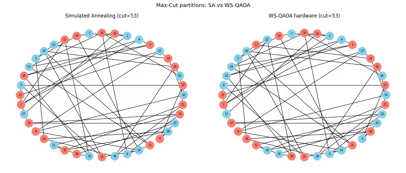
# Visualize both solutions side-by-side on the graph.
# Blue = partition S, orange = partition S-bar.
# Edges crossing between colors are the ones counted in the cut.
fig, axes = plt.subplots(1, 2, figsize=(14, 6))
for ax, assignment, cut, title in [
    (
        axes[0],
        list(sa_solution),
        sa_cut,
        f"Simulated Annealing (cut={sa_cut})",
    ),
    (
        axes[1],
        [int(b) for b in best_bs_hw[::-1]],
        cut_val_hw,
        f"WS-QAOA hardware (cut={cut_val_hw})",
    ),
]:
    colors = [
        "skyblue" if assignment[i] == 0 else "salmon" for i in G_large.nodes()
    ]
    nx.draw(
        G_large,
        pos_large,
        with_labels=True,
        node_color=colors,
        node_size=400,
        font_size=7,
        ax=ax,
    )
    ax.set_title(title)
plt.suptitle("Max-Cut partitions: SA vs WS-QAOA", fontsize=13)
plt.tight_layout()
plt.show()

# ── Step 4: Convergence plot and summary ──────────────────────────────────
# On real hardware the trace will be noisy (shot noise + gate errors), but the
# overall downward trend confirms that COBYLA is making progress despite noise.
fig, ax = plt.subplots(figsize=(7, 4))
ax.plot(ws_history_hw, color="tab:orange", label="WS-QAOA (hardware)")
ax.axhline(
    ws_result_hw.fun,
    color="tab:orange",
    linestyle=":",
    label=f"Final energy ({ws_result_hw.fun:.3f})",
)
ax.set_xlabel("Optimizer call")
ax.set_ylabel(r"$\langle H_C \rangle$")
ax.set_title(f"WS-QAOA convergence on {backend.name} (40 qubits, p=1)")
ax.legend()
plt.tight_layout()
plt.show()

print("\n=== Large Scale Summary ===")
print(f"{'Metric':<38} {'Value':>10}")
print("-" * 50)
print(f"{'Nodes / Edges':<38} {N_LARGE:>5} / {len(edges_large):<4}")
print(f"{'QAOA layers (p)':<38} {p_large:>10}")
print(f"{'Transpiled ECR gate count':<38} {ecr_count:>10}")
print(f"{'Transpiled circuit depth':<38} {ws_isa_large.depth():>10}")
print(f"{'Optimizer iterations':<38} {len(ws_history_hw):>10}")
print(f"{'WS-QAOA energy (hardware)':<38} {ws_result_hw.fun:>10.4f}")
print(f"{'Cut value':<38} {cut_val_hw:>10}")
print(f"{'Simulated annealing cut value':<38} {sa_cut:>10}")
print(f"{'Approximation ratio (vs SA)':<38} {approx_ratio_hw:>10.4f}")

Simulated annealing cut value: 53  (classical reference)
  iter  31  <H_C> = -12.4094
Optimization complete: energy=-13.0256, iterations=31
Most-probable bitstring frequency: 4/8192 (0.0%)
WS-QAOA cut: 53  |  SA cut: 53  |  Approximation ratio vs SA: 1.0000

=== Large Scale Summary ===
Metric                                      Value
--------------------------------------------------
Nodes / Edges                             40 / 60  
QAOA layers (p)                                 1
Transpiled ECR gate count                       0
Transpiled circuit depth                      276
Optimizer iterations                           31
WS-QAOA energy (hardware)                -13.0256
Cut value                                      53
Simulated annealing cut value                  53
Approximation ratio (vs SA)                1.0000

الخطوات التالية

توصيات

إذا وجدت هذا العمل مثيراً للاهتمام، فقد تهتم بالمواد التالية:

• طبقات QAOA أعلى: زد p لترى كيف تتحسن كلتا الخوارزميتين بمزيد من طبقات الدارة، وما إذا كانت ميزة WS-QAOA عند العمق المنخفض تستمر.
• إضافة Qiskit لمخطط التحسين: استكشف التوثيق وجرّب نمذجة مسائل توافقية مختلفة، أو استخدام محلّلات مختلفة للتخفيف المتصل.

المراجع

[1] D. J. Egger, J. Mareček, and S. Woerner, "Warm-starting quantum optimization," Quantum, vol. 5, p. 479, 2021. arXiv:2009.10095

[2] E. Farhi, J. Goldstone, and S. Gutmann, "A quantum approximate optimization algorithm," arXiv:1411.4028, 2014.