القطرنة الكمومية القائمة على العينات المجمّعة لـ Hamiltonian نووي

تقدير الاستخدام: 2.5 دقيقة على معالج Heron (ملاحظة: هذا تقدير فقط. قد يختلف وقت التشغيل الفعلي لديك.)

هل تبحث عن نسخة Fortran؟

يعرض هذا الدفتر التنفيذ بلغة Python. تنفيذ Fortran موجود في دليل Fortran المرافق في مستودع التوثيق هذا. تضيف نسخة Python خطوة استرداد تهيئة ذاتية الاتساق، وهو ما لا تقوم به وحدة تشغيل Fortran.

نتائج التعلم

• تعلّم كيف يصبح Hamiltonian لنموذج الصدفة النووي، المجدول في أساس مدارات مقترن بـ $J$، Hamiltonian كيوبتيًا في مخطط $m$، حيث يمثل كل كيوبت حالة جسيم مفرد واحدة.

• ابنِ نموذجًا إثارة غير تبايني وثابتًا تأتي زواياه من نظرية الاضطراب من الرتبة الثانية، بحيث لا توجد حلقة تحسين كلاسيكية.

• قارن بين الإثارات الكيوبتية والفرميونية وقِس كيف يؤثر الاختيار على عمق المجموعة ثنائي الكيوبت.

• شغّل استرداد التهيئة ذاتي الاتساق باستخدام qiskit-addon-sqd عندما تكون الكميات المحفوظة هي أعداد النكليونات، و $M_J$، والتماثل بدلاً من أعداد الإلكترونات والسبين.

• طبّق سير عمل واحد من مسألة 24 كيوبت يمكنك التحقق منها بدقة إلى مسألة 40 كيوبت تضم ما يقرب من مليوني حالة أساس، وهو ما يتجاوز قدرة القطرنة الدقيقة في هذا الدرس.

المتطلبات المسبقة

قبل البدء، راجع المواضيع التالية:

• القطرنة الكمومية القائمة على العينات ومرجع API لإضافة SQD](https://docs.quantum.ibm.com/api/qiskit-addon-sqd).

• القطرنة الكمومية القائمة على العينات لـ Hamiltonian الكيميائي، النظير الخاص بالبنية الإلكترونية لهذا الدرس.

• الترجمة مقابل هدف خلفية ومقدمة إلى البدائيات.

• التكميم الثانوي وتخطيط جوردان-ويغنر.

الخلفية

يعامل نموذج الصدفة النووي النواة كعدد قليل من النكليونات التكافؤية التي تتحرك في مجموعة صغيرة من مدارات الجسيم المفرد فوق نواة خاملة، وتتفاعل من خلال قوة ثنائية الجسيم تجريبية مضبوطة على الأطياف المقاسة. يُستخدم على نطاق واسع في بنية النواة منخفضة الطاقة. تكلفته الحاسوبية توافقية: الأساس هو كل طريقة لتوزيع البروتونات والنيوترونات التكافؤية على الحالات المتاحة، وهذا النمو يحد من مساحات النموذج التي يمكن الوصول إليها بالقطرنة الدقيقة.

القطرنة الكمومية القائمة على العينات المجمّعة (pooled SQD) [1] تقسم تلك المسألة إلى قسمين. تُستخدم دائرة كمومية فقط لاقتراح الحالات الأساسية المهمة. تُقاس في الأساس الحاسوبي، وتُسمّي كل سلسلة ثنائية مقاسة محدّد سليتر واحد. يُبنى Hamiltonian بعد ذلك ويُقطرن كلاسيكيًا في نطاق تلك المحدّدات. ولأن الخطوة الكلاسيكية هي قطرنة دقيقة داخل فضاء فرعي، فإنها تُرجع حدًا أعلى تبايني على طاقة حالة الأرض الحقيقية، ولا يمكن لهذا الحد إلا أن ينخفض مع إضافة المحدّدات.

يجعل هذا التقسيم للعمل الطريقة متسامحة مع الضوضاء، مع قيد مهم. تغيّر الضوضاء أي من المحدّدات التي تقترحها الدائرة. فهي لا تدخل في Hamiltonian الكلاسيكي، لذا لا يمكنها تحريك القيمة الذاتية لفضاء فرعي معين: تُستبعد أو تُصلح اللقطة التي تنتهك كمية محفوظة، واللقطة التي تبقى هي متجه أساس شرعي أيًا كانت كيفية إنتاجه. لذلك تكلّف الضوضاء جودة الفضاء الفرعي، وليس الصحة، والعدد الذي تُبلّغ عنه هو حد أعلى في كلتا الحالتين.

توفر بنية النواة عدة أعداد كمومية دقيقة لتصفية العينات. يجب أن يحمل المحدّد الفيزيائي العدد الصحيح من البروتونات التكافؤية و العدد الصحيح من النيوترونات التكافؤية، وإسقاط الزخم الزاوي الكلي الصحيح $M_J$، والتماثل الصحيح. يمكن التحقق من كل منها باختبار عدد صحيح على سلسلة ثنائية. تعتمد نسبة العينات المرفوضة على القيد ومساحة النموذج.

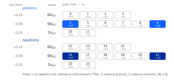
كل كيوبت هو حالة جسيم مفرد واحدة في مخطط $m$ $(n, \ell, j, m_j, t_z)$، و $|1\rangle$ تعني مشغولة. يستخدم السجل ترتيبًا ثابتًا: البروتونات أولًا، ثم النيوترونات؛ ضمن نوع واحد، المدارات بترتيب الملف؛ وضمن مدار واحد، $m_j$ تنازليًا. لذلك يمثل نصفا السلسلة الثنائية تهيئة البروتونات وتهيئة النيوترونات. هذا هو التقسيم الثنائي الذي تتوقعه أدوات المعالجة اللاحقة لـ SQD المجمّعة.

سير العمل

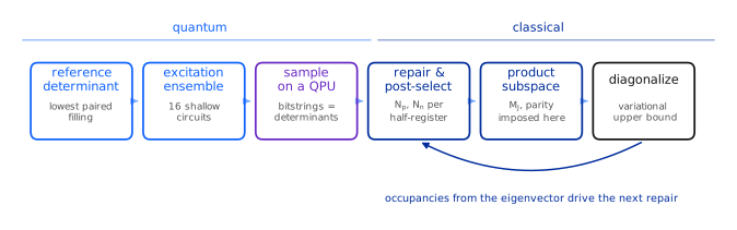
تتعامل مرحلتان في المخطط مع التماثلات النووية.

الإصلاح والانتقاء اللاحق يتعاملان مع العينات المتأثرة بضوضاء العتاد. أعداد النكليونات في نصفي السجل هما وزنا هامنغ، لذا تتعامل qiskit-addon-sqd معهما مباشرة: تُصلح recover_configurations سلسلة ثنائية معطوبة بقلب البتات الأقل اتساقًا مع التقدير الحالي لمتوسط إشغالات المدارات، بدلًا من التخلص من اللقطة.

الفضاء الفرعي الجدائي يُدخل $M_J$. ولأن $M_J = M_p + M_n$ يقرن النصفين، فهو ليس خاصية لأي منهما على حدة، لذلك يجب عدم استخدامه لتصفية اللقطات بأكملها: قد تسهم سلسلة ثنائية نصفها البروتوني ونصفها النيوتروني صالحين كلاهما بنصفي تهيئة جيدين حتى لو كانت $M_J$ الإجمالية خاطئة. لذلك يمتد الفضاء الفرعي بكل جداء لتهيئة بروتونية معاينة مع تهيئة نيوترونية معاينة، مع الاحتفاظ بالجداءات التي تقع في قطاع $M_J$ والتماثل المستهدف. هذا هو بناء الفضاء الفرعي لـ SQD المجمّعة، ويعني أن بضعة آلاف من السلاسل الثنائية يمكن أن تمتد فضاءً فرعيًا أكبر بكثير من عدد العينات.

معادلتان حاكمتان

Hamiltonian نموذج الصدفة هو حد أحادي الجسيم زائد تفاعل ثنائي الجسيم،

$$\begin{equation} \tag{1} H = \sum_{p} \varepsilon_p\, a_p^\dagger a_p + \tfrac{1}{4}\sum_{pqrs} \langle pq \| rs \rangle\, a_p^\dagger a_q^\dagger a_s a_r , \end{equation}$$

حيث تُمثّل $p,q,r,s$ حالات مخطط $m$ و $t_z = -1$ للبروتون، $+1$ للنيوترون. تُجدول التفاعلات التجريبية مثل USDA [2] و GXPF1 [3] ليس في مخطط $m$ بل في الأساس المقترن بـ $J$، كعناصر مصفوفة $\langle ab; J | V | cd; J \rangle$ بين حالتين ثنائيتي الجسيم مضادتي التماثل ومطبّعتين لـ مدارات $a,b,c,d$. استرجاع عنصر مخطط $m$ هو إعادة اقتران كليبش-غوردان،

$$\begin{equation} \tag{2} \langle pq \| rs \rangle = \sqrt{1 + \delta_{ab}}\sqrt{1 + \delta_{cd}} \sum_{J} \langle j_p m_p\, j_q m_q | J M \rangle \langle j_r m_r\, j_s m_s | J M \rangle \langle ab; J | V | cd; J \rangle , \end{equation}$$

مع عوامل $\sqrt{1+\delta}$ التي تُلغي اتفاقية التطبيع للحالات المجدولة. كل شيء آخر في هذا الدرس مبني على هاتين المعادلتين.

عمليات التشغيل الثلاث

	النواة	القشرة	الكيوبتات	الأساس المسموح به تماثليًا	قابل للتحقق دقيقًا؟
صغير النطاق	$^{20}\mathrm{Ne}$ (2p + 2n)	$sd$	24	640	نعم
كبير النطاق	$^{44}\mathrm{Ti}$ (2p + 2n)	$pf$	40	4,000	نعم
كبير النطاق	$^{48}\mathrm{Cr}$ (4p + 4n)	$pf$	40	1,963,461	لا

عملية التشغيل صغيرة النطاق هي الشرح التفصيلي. تستخدم عمليتا التشغيل كبيرتا النطاق كلتاهما سجلًا من 40 كيوبت: الأولى لا تزال صغيرة بما يكفي لقطرنتها بدقة على حاسوب محمول، بحيث يمكنك مقارنة نتيجة العتاد بمرجع دقيق. أما الثانية فتتجاوز قدرة القطرنة الدقيقة لهذا الدرس.

كل عملية تشغيل هنا تُنفَّذ على QPU. هذا خيار اتُّخذ لأجل هذا الدرس وليس متطلبًا من الطريقة نفسها: تشترك عمليات التشغيل الثلاث في خلفية واحدة وميزانية بوابات واحدة بحيث يمكنك مقارنة أدائها عند أحجام مسائل مختلفة.

المتطلبات

ثبّت الحزم التالية قبل البدء:

• Qiskit SDK الإصدار 2.0 أو أحدث (pip install qiskit)

• qiskit-ibm-runtime v0.40 or later (pip install qiskit-ibm-runtime)

• إضافة SQD الإصدار 0.12 أو أحدث (pip install qiskit-addon-sqd)

• NumPy وSciPy وMatplotlib (pip install numpy scipy matplotlib)

تحتاج أيضًا إلى حساب IBM Quantum® ببيانات اعتماد محفوظة محليًا، ووصول إلى QPU يحتوي على 40 كيوبت على الأقل.

لا حاجة لحزمة محاكاة، ولا يجب تنزيل أي ملفات بيانات. ملفا التفاعل اللذان يستخدمهما هذا الدرس مضمّنان في خلية الإعداد التالية ويُكتبان في دليل مؤقت عند تشغيلها.

الإعداد

يستورد هذا القسم الأدوات ويُعرّف مساعدات نموذج الصدفة التي يحتاجها سير العمل، بالترتيب الذي يستخدمها سير العمل به. الفيزياء الكامنة وراء كل منها مشتقة في الملحق؛ تصف التعليقات دور كل دالة في سير العمل.

يُفكّ حزم ملفي تفاعل أولًا. كلاهما مجموعتا معلمات منشورتان، مضمّنتان هنا حتى يكون الدفتر مكتفيًا ذاتيًا: usda.snt هو Hamiltonian قشرة $sd$ الخاص بـ USDA [2] و gxpf1.snt هو Hamiltonian قشرة $pf$ الخاص بـ GXPF1 [3].

# Added by doQumentation — required packages for this notebook
!pip install -q matplotlib numpy qiskit qiskit-addon-sqd qiskit-ibm-runtime scipy

from __future__ import annotations

import base64
import gzip
import itertools
import tempfile
from dataclasses import dataclass
from functools import lru_cache
from math import factorial, sqrt
from pathlib import Path

import matplotlib.pyplot as plt
import numpy as np

from qiskit import QuantumCircuit
from qiskit.circuit.library import PauliEvolutionGate
from qiskit.quantum_info import Operator, SparsePauliOp
from qiskit.transpiler.preset_passmanagers import generate_preset_pass_manager
from qiskit_addon_sqd.configuration_recovery import recover_configurations
from qiskit_addon_sqd.counts import bit_array_to_arrays
from qiskit_addon_sqd.subsampling import postselect_by_hamming_right_and_left
from qiskit_ibm_runtime import QiskitRuntimeService, SamplerV2

from scipy.linalg import eigh

_USDA_SNT_GZ = (
    "H4sIAI5wqWoC/4WY224bRwyG7/UU9F0CONsZco5AUyBuC/QmQNG06KWhWGql1LYMy+kJefiOTrucGXJrQAgsf5nl8ecOr+CX"
    "D9+9g/0K9pv1/T389rx7gPLrsH+Cz/vVctg+vgAsrgB+HeDdAD9t7zYv6+dr+DDA+z8223/X17B8XMFN+ev9+m+4ed799XjA"
    "f9z8sy/4+s8BvoWYrsEERwbhFRqTXi+uCvOwW63vYf+0vFvDAgDo/AFIh8/hK7DH30354Omvb8o3V8c/vIUnMKtboK/wiGKF"
    "+gnFEfVn9PQUe8bthNIRtftbsGfUtQbAGXUFfawM8K0BF9SP6MWA0BpwQcMRvRhwBSX86+fl3ct2d4jq4+eHa3hYv2x2q7fX"
    "AJuPy+fb3cP69+Uh4luAT8djv95++eGV/fj6y6dvFudnmcX4lGOoBmttNOVncTL2FLs3NGT0l++ndJTv0cR8/t6NUanP8WMI"
    "6nPC6C8/5wp+vnn//QLOP9ank3k2wRszkDn/Zwv15xiv41l2SDmjhuEFM4PJ0QkYcgzM4A1Jp1GDkcvtaWMAR9tosAa9huHk"
    "AtoUBYwaF8hGarAxOywgxnoeN+Se2smF4H3QMPZQ653XMJpOi6GyrcLcZJtzLgoYcdsOyXKibV1Aom0fikJO0VLUMDeW3kAl"
    "qQLWpd66qGE02eZ9lXqSPD3UWyl5DeOeGnINJnmaUggCVrtgh2DJNm3fVy8WF3LSMFa9hYga5iYX0IQsYK2nmTpJkoq81Acy"
    "jLTTnPEaxqo3JGcbvZMeGnJVbw6mf2cUqcIsO80nFdOFq8JoSlY+Zb7FfNNZlnw2PqOE8SL3PtlSJhJGXGqsDRjbh4bmocWy"
    "oiIxSxjv09JYgaxlGLZxA9EFFOImuIBt3EB04TK3Z5S8wizrrFCJQ4Xpgl9hzDYbu0LCNm6HzkJHweUkYazITalyF7NjGAnh"
    "FZJFQniFZFHnqWgbdZ6qtoX50VZhvEJ81TJe7AUcQozH8yQMJ8ymUS07jLin6LXT3FRIhmwSTmtbJpEjr2AsvM7E1ra+ZaiM"
    "NoxewZinBlPQTmPJyikn7TQ2630SbWuz4CLlwzuGhCHPqbUmRZQwpkiBDn1vsoQ55oKjbEvNNVgbXls0WvA0NKnPpku91Fkx"
    "pahhXPDJtxVCQkBcMtJD27I8VJGAhWYYlVuZzc5e+jSIZWnLa57nOQ1iWZY+jSE3GP5/QIKi5E1Agqi9BbMZiUjEWNwChqKq"
    "KTZY11ku5ca2Pqc4YKk1o2DstBjJC1htW2nAgEZ4aDdPvQmmmLeY4tWFt9Y3VAdlpW+oDcpa3zpM1jdUB2XV9agOyqrrcWZQ"
    "sq7vMMffBseux5l5yjoLZ+Yp6yzU5mmt5DgzT5mSozZPoVIknJmnTJFQHZRV12OrlvpFQFbycoGKOWiYfl9QlXySGtSUvL9W"
    "VJi/YG4grC4CmuCX6CZrKUsY64UyJolCQoZJqWeKhDOCzxQJNcGXbZMEX7EtzF+gvCI1npxjmKaW5Q06ewVjOY0u2+Y0kt5D"
    "JhlETS2P+5CqyIMYkCI1NK50SO3TarSR2qfVaKOZPmXjg2beVJmS01zqp/CSmvoqvNSOD/kaS+qUoSGaTM2yz83fdjtMvsZy"
    "xOv7N44Fff/GT5q5tXWYfB3jWND3b9yumUvK5SQnvK6w/VuHyfu3DpP3bx0m7984FvT9W4fJ+zceWq/v3zpM3r9xLOj7tw6T"
    "928X053QgGz/1mHy/u3yZ8lTtn/jWND3b74NiDx2vRbeep56Lbz1oPRaeOv9G0dmxofXPK33bx0m798C1B9RuP4DPJ0WcLAa"
    "AAA="
)

_GXPF1_SNT_GZ = (
    "H4sIAI5wqWoC/4WcQY8dtw3H7/kU41sCeF8lUqKkQw9NgbaXoEHQQ26BkdiIEWdt2E6L9tNXb9+ORIn8PwdZILB/S3I4IsW/"
    "ZiYvjr//+P3f4nG8ef/x+PDm4dOvr9+9++rF8d3l+Mf7x99fvTz+dTn++fnTH7/1//z28pfL8e3H9/95fHm8evzl+lffvf3f"
    "H59e/fb26L9zHN//+t9Pl+OH1/++HH89JL88gkQO8esfvjm+phDomyvW//39/S+v3x2fPrz6+fVX/dfS889B4fpz/aN43P7p"
    "f3Bw/ynH8fD0Zy+uf/fn48MR3vxU/kRXlp7Z+PzDiqUnNn74iW8sb3azYvm0m29s2uxGxabTbryx2cZ7nGzu7KOKV2y8g5Un"
    "dsZbbLyDLafd53irjXew9bR7jffF8fbx8+uPr37+/Pb941dPv3P93ZH4W/If6kUohXCm+Jbmh3yR0jicybwl9CFeuFILy908"
    "HtIlcrlZyCNJ2q6MdGi7ZVy4tlvHJS52Y71FnHp8D+HCIYTlQuYFhdsv0yVxzZB6vsxwaZwJUumkIjWB1POdDhcqlR2KVo85"
    "SoDU8NgdNodiZevqMUqB1LCVWsO2ZMQlyYs+bXEFk4m5bMJJlVgSpGjaouhQvFKxUIbUjIvI85hWW4FNvubyDnMxMkFKRc8V"
    "Uml65OhQW1x9fe3XOAtsZPXJ36TIX18SaoQUnysnZsHUXPfcKqTyaSu36FHbWg0tN0jxWIXEAVLzbqcqkMpj3T8lwlBp9RhD"
    "qpAaHpnzni9nRXPh6lDbysmJBVLzDtU71KztnDxqW1+JhDaKnTtUa4DUzH00Hp0VXQMHSM3c16irlpf7GEcN1dogpfpEDpAa"
    "WRUOBKl0UqkIQ2qs+5IYU6OvthbFodIaF6/9i51VeF0TLZSN2lfh9T729utQOqtXKi/dl/21mihhW+M+BpIKqblypDWHSntc"
    "mSA1O3nMe+6dHp0DEaRmXCU0h9p7dOYCqVm1MehOnvy7nWphSKnuu+Q++X2Ca4uQGrYkxp3yMkFLL0ygavPovmR64dhFY5QM"
    "KVK1XRxqX4UydlHCXU44hY1ydndKuUBK11BzqH1NNOKNMvt27PMXVUWBemSqCVIjrr4nYFtzTSQJkJp3O7se09p9YygCKVL7"
    "UN4opx5DNnE5q5AlerZ2jyExpEYmggTtMYFrzC1Bak58jetGeSvHenSip9ROik0m5lqdsxzjrCYhTM1uImOHYZzVPvnWjXIm"
    "0RoaKyqhjjlqiEE3uWoYHqopbT/KY0pDD+Xtx9d8lvI0n6U8zWcpT/NpQqDms5Sn+TRVoOazlKf5LOVpPk1VqPl05AI1n6U8"
    "zaepAjWfpTzNp6kKNZ/OQoGaz1Ke5rOUp/k0VaHm03mvUPOd1+esL6X5LOVpPkt5ms9SnubTVIGaz1Ke5rOUp/ks5Wk+TVWo"
    "+SzlaT69mgVqPk0VqPks5Wk+S3maT1MVaj5dPwVqPkt5mk9TFWo+S3ma77x/8z56ms9SnuazlKf5LOVpPkt5ms9SnubTVIWa"
    "z1Ke5jupfRWumk9TBWo+S3maz1Ke5rOUp/k0VaHms5Sn+XTnLVDzWcrTfJqqUPNZytN85/1z7rbSfJbyNN/5t06fUJrPUp7m"
    "OykvE7T0wgqqdmo+Mb3Q03yCO6bSfII7ptJ8gruc0nxi+pen+eROL5yaT3CXU5pPx1Sh5hNcj0rzCajHVfMJqMdV88mdesyu"
    "xwo1n+B6VJpPcD0qzSe4HpXmE1yPSvMJrkelwERVR4Waz1Ke5hNTQ3THoxO90nzFZMLTfAVnVWm+grOqNF/BWVWaTxMVar6C"
    "r1FpvgK6yar56vbja76onormu8/5ViqOrNblZH6l0NPAlRq9sKaIbaFnhis15tUuH/E1oieLK1XOTIgsz3ROap9XpQ/SJWqK"
    "bCYcKm6K4tp9iUqqzbd1j4qO+g2tpTV6sll1qLipk6fnw32/isDWPSruPborwz7x9eakKbbry6Gi7RN9nrhuHr4tPXXsVLT9"
    "vvTdKlUQ18i9Q0Wn+2ZOlYpva0yiDhXthNz69p4S+7ZG7h0q2jma+/BIIfm2RnU4VLQ9R6hG4iWryVurhorOlNbzEJr4tubk"
    "bim6e25iqbFbJY4MKfREfaXGNXKK2aF2BSapD6Oy5162yd1S5Og0iq3k5tua1WEpsus+ZO4ZS76tqU4sRc7+mAtJyL6teR8t"
    "RVbDUO9yXM2a2O6jQ5GjdCi3HKpva04dluK7J1uWGtFLjhFS6J2HlZpKhzOm0JsRK5XnmjD7Izv5av0eBd7zVb5IsVU6ffTN"
    "oQXf1peoeveNjZWaNURFZ0L8fTsX1s9hwO4eeHkOA3Z3Zct6ZOccgPAM0O91hR4ZPEcWMAPkdBWQvsdZj72xZuTRs2U95qFY"
    "a8FZHVQpy/Mhd55YbGmPew2VGB2PRvOVsNlib0orYbO1U8fi0cbF6uQhw7jUycMybYs/dSiKwGxyLB5tXEmdM5WM4lKnGLFm"
    "FFeaPTruK8ehlEcbV55n2yIwrnlOXorAuPKsxyIwrjz7l3greptzSgve+tqo2lLbcu9MQ4oiPDMpjzaueR8rUUZxqaql/T46"
    "k5WiCM9fyuNpy5uZpM9WkvfaxpS1Ndd96JKV2LflUdrW1idaKOT0HNMnTCdnT/OZvcOZv5RHG5fqAJFhXLO2WykwrtlzJkV4"
    "llMebVxp7kOUMopr7h1dSmcUl9LuxesT2z6kPOq4ttkkk7sj1/1JWWWnHvfdfVKE50LlUV+jObPqs2hO+zViytpSJ+CFSyu+"
    "LY+yttRM3gf3HH1bHmVtzR5NXZQXcI0epW1tdyh2d86a2O52F9vR6V8FUgTm1dWjjWuepZUgMK45k2cKMC6PIjD7rh6j+gpi"
    "0Y904b675/n2h3u6QteTedkoc7qy2LIeaUxpkXNAHgeV53khozOYxZb1qDpTrvAa+TxBClECvEbPlvWY5o4cA7zGNDSfFIbX"
    "6NmyHmd1SEnwGgfVJ6YKr9GzZT3KebdDZIYe5bzGQLFAj54t7XHXfDkmJ6v789r17e7iTEMrxXhmUh5tXHNmainCuObMVBOO"
    "y6MYzEyrx9MW2VMf4cC9NWlbzpmVoqytucPkIO12SsZ4/lKUtTX7V6LGsfi2phadlLa1nX89naUHc437uYnQni/nlEzWN/S8"
    "s7TVo41LvUsW9+pwqFBl79HsPYkVr/sK9GjjYnVWSzBfqjoowXx5FN+ZC6dHG5d6WybjfM15ouYE8+VRDObC1aOOa3v+WEJq"
    "Tlzb2VCRELOtbYEU47NH5dHGpd5nagzj0s+HAozLoxjMq6tHnfutHmNjblz23G/1qChra3rMOT6f3jGefRVlbamZKfR1COKa"
    "PWdS1tZcXy3mnMm3pd4IGpS1Nd9Uai0Wir6t+fxxUtrWPvu27M1MG8XJ1KMz+yqK8Vmt8mjjmn1CKmcUF88zhVIzimtOtZNi"
    "fO6rPGpbW9XGLrg50G5rfwNhUueu7swmEtI55yQ0m/RpqI3JPd15ujVtWY9TSbcxpSU8dSShAj16tk4b3r6dmUlI2/L27Ulp"
    "W7vKLFK3uByK4nI2VP19SFEJ7EOrRxvXyESr413YhPchLsssV/0dRlEJ70PKo7a1n/vWa1rLbsu8mTooa0up8tpyEd+Wep42"
    "KG1rf6su5ebkvpqztLzl3qltRSVc28ojmTM+9F2TwNm3Qgp9/eSeKnaNXFtwqH3nk1KaJE05M6ZDOdNjv9NJIvm2Zr+3lFeP"
    "EvqGnH1bM/eWMtNQvFCRHnzUlJlzXMqZYFKqHHLxbdFUFIbiu+8XWmo+50vL6R06l1u/PBO/asN8B5zAmdXTDtP7r8h+jeWL"
    "lFOPocYumti39SWq3v0iTvxdtDw9hhmUq9N6PbaqvzJyqyNeMi0nIm51LLbojgIrOUKP+l2yBj16tghrqxib1gqg0pLknfIq"
    "bdoirJqkMMNrnDNATPgaPVuE9VBv0J7HbU107V42W44eUhSjPrF4JKyHUokZxqXeTV+exAI9pCjGp/zKIwE9dO2+XSTX1vbc"
    "b6pJUYT1UOCWWw2+rdmZJkVYD1Ef0Uoi39acySdFWA9RztLVjm9LPQ0cFAENc3unJjrVsWuY0mK297EYxbrbcs7vlUfCGib3"
    "bQ/GNWffMijCGkZRDHr0w+KRsIbpnem6dnZbe9VOitTsW7e3I+e7Pgnv7tfHQxvl7O7KlvU4zu95fouUUNV21RSGFk2oHhdb"
    "ZGbf+b4cXf8nRlnb8maASVlbc+UkSnSb0hKox4eFIjNHz7c/aHydkvC6T9Lydo3Je+u8ZSdf+xsu06O2ta2vPr70W1l2W9v6"
    "UhSbPoG+kwYnSDVnTKGvqYvfv3JuDVLom2vvpOZpvh9fizHuX71jVp79vqDcG8rrJolLnecTxe8TgMLfBTDoJteOGUVntYJr"
    "5PHOVsKnUaEuJw8oE9MWA5V5e2tA9wmQrw5xQB6RrernS33VkEB1PCmKW5f7P6zudeW7TwAA"
)

DATA = Path(tempfile.mkdtemp(prefix="nuclear_sqd_"))
for name, blob in (("usda.snt", _USDA_SNT_GZ), ("gxpf1.snt", _GXPF1_SNT_GZ)):
    (DATA / name).write_bytes(gzip.decompress(base64.b64decode(blob)))

    if not (DATA / name).is_file():
        raise RuntimeError(f"{name} did not unpack to {DATA}")

مساحة النموذج وسجل الكيوبتات

يحتوي ملف .snt على مساحة النموذج، وطاقات الجسيم المفرد، وعناصر المصفوفة الثنائية المقترنة بـ $J$. بالنسبة للتفاعلات المعتمدة على الكتلة المستخدمة هنا، يحدد الحقلان الثالث والرابع من رأس الجزء الثنائي الكتلة المرجعية $A_{\mathrm{ref}}$ التي جرى ضبط التفاعل عندها وأس اعتماده على الكتلة. يحمل كلا الملفين الأس $-0.3$، مع $A_{\mathrm{ref}} = 18$ لـ USDA و $42$ لـ GXPF1، لذا يجب إعادة قياس عناصر المصفوفة المجدولة بمقدار $(A/A_{\mathrm{ref}})^{-0.3}$ للنواة قيد الحساب [2]، [3]. لا يُعاد قياس طاقات الجسيم المفرد. تخطي هذه الخطوة يغيّر طاقة الترابط ببضع نسب مئوية.

الطاقات التالية هي طاقات تكافؤ، تُقاس من النواة الخاملة؛ وليست طاقات انفصال تجريبية.

@dataclass(frozen=True)
class Orbital:
    idx: int
    n: int
    ell: int
    j2: int
    tz: int  # j2 = 2j; tz = -1 proton, +1 neutron

@dataclass(frozen=True)
class SPState:
    """One m-scheme single-particle state, i.e. one qubit."""

    orb: int
    j2: int
    mj2: int
    tz: int
    ell: int
    spe: float  # mj2 = 2 * m_j

@dataclass
class ModelSpace:
    orbitals: list
    spes: dict
    tbmes: dict
    core_z: int
    core_n: int
    mass_number: int
    a_ref: int
    mass_exponent: float
    mass_factor: float

def read_snt(path, n_protons, n_neutrons):
    """Parse a .snt interaction file, applying its mass dependence for this nucleus.

    The two-body header line is ``n_tbme  method  A_ref  exponent``.  When ``method`` is 1 the
    tabulated matrix elements are rescaled by ``(A / A_ref) ** exponent``, where A is the mass
    number of the whole nucleus -- the core plus the valence nucleons.  A is derived from the
    file's own core numbers rather than passed in, so it cannot silently disagree with the
    valence counts the rest of the workflow uses.  Single-particle energies are not rescaled.
    """
    rows = [
        ln.split("!")[0].split() for ln in Path(path).read_text().splitlines()
    ]
    rows = iter([r for r in rows if r])

    n_p_orb, n_n_orb, core_z, core_n = (int(x) for x in next(rows)[:4])
    orbitals = [
        Orbital(*(int(x) for x in next(rows)[:5]))
        for _ in range(n_p_orb + n_n_orb)
    ]

    spes = {}
    for _ in range(int(next(rows)[0])):  # "i  i  <i|H(1b)|i>"
        field = next(rows)
        spes[int(field[0])] = float(field[2])

    n_tbme, method, a_ref, exponent = next(rows)[:4]
    n_tbme, method, a_ref, exponent = (
        int(n_tbme),
        int(method),
        int(a_ref),
        float(exponent),
    )
    mass_number = core_z + core_n + n_protons + n_neutrons
    factor = (mass_number / a_ref) ** exponent if method == 1 else 1.0

    tbmes = {}
    for _ in range(n_tbme):  # "a  b  c  d  J  value"
        field = next(rows)
        tbmes[tuple(int(x) for x in field[:5])] = float(field[5]) * factor

    return ModelSpace(
        orbitals,
        spes,
        tbmes,
        core_z,
        core_n,
        mass_number,
        a_ref,
        exponent,
        factor,
    )

def m_scheme_states(ms):
    """The qubit register: protons then neutrons, orbitals in file order, m_j descending."""
    return [
        SPState(o.idx, o.j2, m2, o.tz, o.ell, ms.spes[o.idx])
        for tz in (-1, +1)
        for o in ms.orbitals
        if o.tz == tz
        for m2 in range(o.j2, -o.j2 - 1, -2)
    ]

إعادة اقتران كليبش-غوردان

تتطلب المعادلة (2) معاملات كليبش-غوردان لأزخام زاوية نصف صحيحة. تُمرَّر كل وسيطة بوصفها ضعف قيمتها الفيزيائية، لذا يُدخَل $j = 5/2$ كـ 5 ويبقى الحساب دقيقًا.

تتعامل Interaction.v_ms مع عمليات البحث عن عناصر مصفوفة التفاعل. يخزّن ملف .snt كل عنصر مصفوفة مرة واحدة، لذا قد يحتاج البحث إلى طور تبادل الزوج المضاد للتماثل $-(-1)^{j_a + j_b - J}$ على أي جانب، وقد يُخزَّن البرا والكيت بأي ترتيب.

@lru_cache(maxsize=None)
def clebsch_gordan(j1_2, j2_2, J_2, m1_2, m2_2, M_2):
    """<j1 m1 j2 m2 | J M>.  Every argument is twice its physical value."""
    if m1_2 + m2_2 != M_2 or not abs(j1_2 - j2_2) <= J_2 <= j1_2 + j2_2:
        return 0.0
    if abs(m1_2) > j1_2 or abs(m2_2) > j2_2 or abs(M_2) > J_2:
        return 0.0
    if (j1_2 + j2_2 - J_2) % 2 or (j1_2 - m1_2) % 2 or (j2_2 - m2_2) % 2:
        return 0.0

    f, half = factorial, lambda x: x // 2
    prefactor = sqrt(
        (J_2 + 1)
        * f(half(j1_2 + j2_2 - J_2))
        * f(half(j1_2 - j2_2 + J_2))
        * f(half(-j1_2 + j2_2 + J_2))
        / f(half(j1_2 + j2_2 + J_2) + 1)
        * f(half(J_2 + M_2))
        * f(half(J_2 - M_2))
        * f(half(j1_2 - m1_2))
        * f(half(j1_2 + m1_2))
        * f(half(j2_2 - m2_2))
        * f(half(j2_2 + m2_2))
    )
    total = 0.0
    for k in range(half(j1_2 + j2_2 - J_2) + 1):
        d = [
            half(j1_2 + j2_2 - J_2) - k,
            half(j1_2 - m1_2) - k,
            half(j2_2 + m2_2) - k,
            half(J_2 - j2_2 + m1_2) + k,
            half(J_2 - j1_2 - m2_2) + k,
        ]
        if all(x >= 0 for x in d):
            total += (-1) ** k / (
                f(k) * f(d[0]) * f(d[1]) * f(d[2]) * f(d[3]) * f(d[4])
            )
    return prefactor * total

class Interaction:
    """Antisymmetrized m-scheme two-body matrix elements <pq||rs>, per Eq. (2)."""

    def __init__(self, model_space, sp):
        self.ms, self.sp, self._cache = model_space, sp, {}

    def _tbme(self, oa, ob, oc, od, J, j_ab_2, j_cd_2):
        """<oa ob; J|V|oc od; J>, allowing for how the file happens to order each pair."""
        table = self.ms.tbmes
        # |ba; J> = -(-1)^(j_a + j_b - J) |ab; J> for a normalized antisymmetrized pair;
        # dropping the leading minus makes v_ms symmetric instead of antisymmetric, and
        # the Hamiltonian then fails the rotational-invariance check in Step 1.
        phase_ab = -1.0 if (j_ab_2 // 2 - J) % 2 == 0 else 1.0
        phase_cd = -1.0 if (j_cd_2 // 2 - J) % 2 == 0 else 1.0
        for keys, phase in (
            (((oa, ob, oc, od), (oc, od, oa, ob)), 1.0),
            (((ob, oa, oc, od), (oc, od, ob, oa)), phase_ab),
            (((oa, ob, od, oc), (od, oc, oa, ob)), phase_cd),
            (((ob, oa, od, oc), (od, oc, ob, oa)), phase_ab * phase_cd),
        ):
            for key in keys:
                value = table.get(key + (J,))
                if value is not None:
                    return value * phase
        return 0.0

    def v_ms(self, p, q, r, s):
        """<pq||rs>, zero unless M_J and charge are conserved."""
        cached = self._cache.get((p, q, r, s))
        if cached is not None:
            return cached

        P, Q, R, S = (self.sp[i] for i in (p, q, r, s))
        value = 0.0
        if P.mj2 + Q.mj2 == R.mj2 + S.mj2 and P.tz + Q.tz == R.tz + S.tz:
            M = P.mj2 + Q.mj2
            # sqrt(1 + delta): undo the normalization of the tabulated pair states
            c12 = sqrt(2.0) if (P.tz == Q.tz and P.orb == Q.orb) else 1.0
            c34 = sqrt(2.0) if (R.tz == S.tz and R.orb == S.orb) else 1.0
            for J2 in range(
                max(abs(P.j2 - Q.j2), abs(R.j2 - S.j2)),
                min(P.j2 + Q.j2, R.j2 + S.j2) + 1,
                2,
            ):
                cg_bra = clebsch_gordan(P.j2, Q.j2, J2, P.mj2, Q.mj2, M)
                cg_ket = clebsch_gordan(R.j2, S.j2, J2, R.mj2, S.mj2, M)
                if abs(cg_bra) < 1e-12 or abs(cg_ket) < 1e-12:
                    continue
                value += (
                    c12
                    * c34
                    * cg_bra
                    * cg_ket
                    * self._tbme(
                        P.orb,
                        Q.orb,
                        R.orb,
                        S.orb,
                        J2 // 2,
                        P.j2 + Q.j2,
                        R.j2 + S.j2,
                    )
                )

        self._cache[(p, q, r, s)] = value
        return value

عناصر المصفوفة واختبار التماثل

المحدّد هو مجموعة مرتبة من فهارس الكيوبتات المشغولة. المحدّدان اللذان يختلفان في أكثر من حالتين مشغولتين لهما عنصر مصفوفة متلاشٍ؛ وإلا، تعطي قواعد سليتر-كوندون مجموعًا قصيرًا على التفاعل، مضروبًا في إشارة فرميونية تحسب عدد الحالات المشغولة الواقعة بين المؤثرين في ترتيب السجل الثابت.

symmetry_allowed هو اختبار العدد الصحيح الذي تختزل إليه جميع الأعداد الكمومية الدقيقة الأربعة. يُستخدم كلًا من تصفية العينات وتعداد الأساس الدقيق لعمليات التشغيل الصغيرة بما يكفي للتحقق.

def matrix_element(inter, det_a, det_b):
    """<A|H|B> for two determinants, each a sorted tuple of occupied qubit indices."""
    set_a, set_b = set(det_a), set(det_b)
    out_a, out_b = sorted(set_a - set_b), sorted(set_b - set_a)
    if len(out_a) != len(out_b) or len(out_a) > 2:
        return 0.0

    if not out_a:  # diagonal: one-body plus two-body
        return sum(inter.sp[i].spe for i in det_a) + sum(
            inter.v_ms(i, j, i, j)
            for i, j in itertools.combinations(det_a, 2)
        )

    if len(out_a) == 1:  # one state moves, p -> q
        p, q = out_a[0], out_b[0]
        crossings = sum(1 for k in set_a if min(p, q) < k < max(p, q))
        return (-1.0) ** crossings * sum(
            inter.v_ms(p, j, q, j) for j in det_a if j not in (p, q)
        )

    (p, r), (q, s) = out_a, out_b  # two states move
    crossings = sum(1 for k in set_a if p < k < r) + sum(
        1 for k in set_b if q < k < s
    )
    return (-1.0) ** crossings * inter.v_ms(p, r, q, s)

def subspace_hamiltonian(inter, dets):
    """Dense real-symmetric H projected onto the span of `dets`."""
    H = np.zeros((len(dets), len(dets)))
    for a, det_a in enumerate(dets):
        H[a, a] = matrix_element(inter, det_a, det_a)
        for b in range(a + 1, len(dets)):
            H[a, b] = H[b, a] = matrix_element(inter, det_a, dets[b])
    return H

def ground_state(inter, dets):
    """Lowest eigenvalue and eigenvector of H over `dets`."""
    values, vectors = np.linalg.eigh(subspace_hamiltonian(inter, dets))
    return values[0], vectors[:, 0]

def symmetry_allowed(
    sp, det, n_protons, n_neutrons, mj2_target=0, parity_target=0
):
    """The four exact shell-model quantum numbers, as integer tests on one determinant."""
    n_p = sum(1 for i in det if sp[i].tz == -1)
    return (
        n_p == n_protons
        and len(det) - n_p == n_neutrons
        and sum(sp[i].mj2 for i in det) == mj2_target
        and sum(sp[i].ell for i in det) % 2 == parity_target
    )

def full_basis(sp, n_protons, n_neutrons, **targets):
    """Every symmetry-allowed determinant.  Only tractable for small model spaces."""
    protons = [i for i, s in enumerate(sp) if s.tz == -1]
    neutrons = [i for i, s in enumerate(sp) if s.tz == +1]
    return [
        p + n
        for p in itertools.combinations(protons, n_protons)
        for n in itertools.combinations(neutrons, n_neutrons)
        if symmetry_allowed(sp, p + n, n_protons, n_neutrons, **targets)
    ]

def count_basis(sp, n_protons, n_neutrons, mj2_target=0, parity_target=0):
    """How many determinants `full_basis` would return, without enumerating them.

    A dynamic program over (occupied count, sum of 2*m_j, parity) per species.  This stays
    cheap when the basis itself is far too large to build, which is how the largest run below
    can report the size of the space it is sampling from.
    """

    def species(states, k):
        table = {(0, 0, 0): 1}
        for s in states:
            for key, value in list(table.items()):
                count, m_sum, parity = key
                if count < k:
                    nxt = (count + 1, m_sum + s.mj2, (parity + s.ell) % 2)
                    table[nxt] = table.get(nxt, 0) + value
        totals = {}
        for (count, m_sum, parity), value in table.items():
            if count == k:
                totals[(m_sum, parity)] = (
                    totals.get((m_sum, parity), 0) + value
                )
        return totals

    left = species([s for s in sp if s.tz == -1], n_protons)
    right = species([s for s in sp if s.tz == +1], n_neutrons)
    return sum(
        a * b
        for (mp, pp), a in left.items()
        for (mn, pn), b in right.items()
        if mp + mn == mj2_target and (pp + pn) % 2 == parity_target
    )

المحدّد المرجعي

يُبنى النموذج فوق محدّد واحد، لذا يجب أن يكون ذلك المحدّد هو الأفضل المتاح. ملء طاقات الجسيم المفرد الأدنى يتجاهل التفاعل الثنائي. في مساحات النموذج هذه، يعطي هذا الاختيار طاقة أعلى بمقدار 1-2 MeV من المحدّد الأدنى طاقة.

يفرض التقييد بالتعبئات المكوّنة من أزواج معكوسة زمنيًا $(+m_j, -m_j)$ قيمة $M_J = 0$ تمامًا ويترك فقط $\binom{n_{\mathrm{pairs}}}{k}$ مرشحًا لكل نوع (بضعة آلاف على الأكثر)، لذا يمكن إيجاد الأفضل بالبحث عنها جميعًا على القطر الكامل $\langle \Phi | H | \Phi \rangle$. في حالات التعادل، يُرجَّح الأزواج الأكثر محاذاة قوية، حيث تكون قوة اقتران $J = 0$ الأقوى. في كل حالة في هذا الدرس يمكن التحقق منها مقابل تعداد كامل، يُرجع البحث المحدّد الأدنى قطريًا عالميًا، والذي يمثل أيضًا أكبر مكوّن مفرد في حالة الأرض الدقيقة.

def reference_determinant(sp, inter, n_protons, n_neutrons):
    """Lowest-diagonal determinant built from time-reversed (+m_j, -m_j) orbital pairs."""
    if n_protons % 2 or n_neutrons % 2:
        raise ValueError(
            "an odd valence count has no time-reversed paired reference at M_J = 0"
        )

    def species_pairs(tz):
        return [
            (
                q,
                next(
                    p
                    for p, t in enumerate(sp)
                    if t.tz == tz and t.orb == s.orb and t.mj2 == -s.mj2
                ),
            )
            for q, s in enumerate(sp)
            if s.tz == tz and s.mj2 > 0
        ]

    best = None
    for chosen_p in itertools.combinations(species_pairs(-1), n_protons // 2):
        protons = tuple(q for pair in chosen_p for q in pair)
        for chosen_n in itertools.combinations(
            species_pairs(+1), n_neutrons // 2
        ):
            det = tuple(
                sorted(protons + tuple(q for pair in chosen_n for q in pair))
            )
            # break ties toward the most aligned pairs, where J = 0 pairing is strongest
            score = (
                matrix_element(inter, det, det),
                -sum(abs(sp[q].mj2) for q in det),
            )
            if best is None or score < best[0]:
                best = (score, det)
    return best[1]

مجموعة الإثارات وترتيبها الاضطرابي

يُحمَل الترابط بإثارات جسيمين-ثقبين ($2p2h$) من المرجع. تُقلّل قاعدتا اختيار حجم المجموعة قبل بناء أي دائرة: يجب أن تحفظ الإثارة $M_J$، ويجب أن يتمكن زوج الثقوب وزوج الجسيمات من الاقتران بـ $J$ إجمالي مشترك، وهو متباينة مثلثية.

تُرتَّب الإثارات المتبقية حسب نتيجة إبستين-نيسبت من الرتبة الثانية للتفاعل التكويني المختار [4]،

$$\begin{equation} \tag{3} s_\alpha = \frac{|\langle \Phi_{\mathrm{ref}} | H | \alpha \rangle|^2}{|\Delta_\alpha|}, \qquad \Delta_\alpha = H_{\mathrm{ref},\mathrm{ref}} - H_{\alpha\alpha}, \end{equation}$$

والتي تُقدِّر مقدار طاقة الترابط التي تحملها كل إثارة. يحدد نفس الرقمين زاوية الدائرة: مع $V = \langle \Phi_{\mathrm{ref}} | H | \alpha \rangle$، سعة الرتبة الأولى هي $t_\alpha = V / \Delta_\alpha$. يشرح الملحق لماذا سعة الرتبة الأولى هي الاختيار المستخدم في هذا الدرس بدلًا من زاوية المستويين الدقيقة.

def excitation_pool(sp, occ):
    """2p2h quadruples (h1, h2, v1, v2): same-species pairs, then proton-neutron pairs."""
    holes = {tz: [i for i in occ if sp[i].tz == tz] for tz in (-1, +1)}
    virtuals = {
        tz: [i for i, s in enumerate(sp) if s.tz == tz and i not in occ]
        for tz in (-1, +1)
    }
    pool = [
        (h1, h2, v1, v2)
        for tz in (-1, +1)
        for h1, h2 in itertools.combinations(holes[tz], 2)
        for v1, v2 in itertools.combinations(virtuals[tz], 2)
    ]
    pool += [
        (h1, h2, v1, v2)
        for h1 in holes[-1]
        for h2 in holes[+1]
        for v1 in virtuals[-1]
        for v2 in virtuals[+1]
    ]
    return pool

def conserves_symmetry(sp, op):
    """Keeps M_J, and the hole and particle pairs share a reachable total J."""
    h1, h2, v1, v2 = op
    if sp[v1].mj2 + sp[v2].mj2 != sp[h1].mj2 + sp[h2].mj2:
        return False
    return max(abs(sp[v1].j2 - sp[v2].j2), abs(sp[h1].j2 - sp[h2].j2)) <= min(
        sp[v1].j2 + sp[v2].j2, sp[h1].j2 + sp[h2].j2
    )

def en_denominator(inter, occ, holes, virtuals, floor=0.1):
    """Epstein-Nesbet gap: bare gap, spectator rearrangement, and the pair's own term."""
    gap = sum(inter.sp[h].spe for h in holes) - sum(
        inter.sp[v].spe for v in virtuals
    )
    for k in occ:
        if k in holes:
            continue
        gap += sum(inter.v_ms(h, k, h, k) for h in holes)
        gap -= sum(inter.v_ms(v, k, v, k) for v in virtuals)
    gap += inter.v_ms(holes[0], holes[1], holes[0], holes[1])
    gap -= inter.v_ms(virtuals[0], virtuals[1], virtuals[0], virtuals[1])
    return gap if abs(gap) >= floor else (floor if gap >= 0 else -floor)

def rank_pool(inter, occ, pool):
    """Sort by descending PT2 score; return (operator, coupling, first-order amplitude)."""
    ranked = []
    for op in pool:
        h1, h2, v1, v2 = op
        coupling = inter.v_ms(v1, v2, h1, h2)
        gap = en_denominator(inter, occ, (h1, h2), (v1, v2))
        ranked.append((coupling**2 / abs(gap), op, coupling, coupling / gap))
    ranked.sort(key=lambda row: (-row[0], row[1]))  # deterministic on ties
    return [
        (op, coupling, amplitude) for _, op, coupling, amplitude in ranked
    ]

كتل الإثارة الكيوبتية

تحت تخطيط جوردان-ويغنر، يصبح مؤثر إثارة $2p2h$ الحافظ للجسيمات مجموعًا من ثماني سلاسل باولي، تحمل كل منها سلسلة من مؤثرات $Z$ بين الفهارس الخارجية. تفرض سلاسل $Z$ عدم التماثل الفرميوني، وهي مكلفة: تمتد إثارة بروتون-نيوترون عبر الحدود بين نصفي السجل وتتضمن سلسلة تماثل عبر تلك الحدود.

إسقاط سلاسل $Z$ يعطي مؤثر الإثارة الكيوبتية لـ Yordanov وزملائه [5]. للحالة التي يحضّرها هذا المؤثر سعات مختلفة، لكنه يصل بالضبط إلى نفس أزواج المحدّدات، لذا تبقى مجموعة المحدّدات التي يمكن للدائرة الوصول إليها دون تغيير. تستخدم SQD المجمّعة هذه المحدّدات للقطرنة الكلاسيكية. تقارن الخطوة 2 دعم البنيتين وتقيس تكاليف العتاد الخاصة بهما.

بناء صيغة باولي من $a_j^\dagger = \tfrac{1}{2}(X_j - i Y_j) \otimes Z_{<j}$، مع كون سلسلة $Z$ اختيارية، يبقي البنيتين متفاصلتين بعلامة واحدة فقط. جميع الحدود الثمانية لمولّد واحد تتبادل، لذا فإن خطوة PauliEvolutionGate واحدة هي الأسية الدقيقة وليست تقريب تروتر لها.

def _ladder(num_qubits, q, dagger, parity):
    """Pauli form of a_q or a_q^dagger.  `parity` toggles the Jordan-Wigner Z string."""
    prefix = (
        ["Z"] * q + ["I"] * (num_qubits - q) if parity else ["I"] * num_qubits
    )
    x_part, y_part = list(prefix), list(prefix)
    x_part[q], y_part[q] = "X", "Y"
    return SparsePauliOp(
        ["".join(reversed(x_part)), "".join(reversed(y_part))],
        coeffs=[0.5, 0.5 * (-1j if dagger else 1j)],
    )

def excitation_generator(num_qubits, op, parity=False):
    """Hermitian H with exp(-i theta H) = exp(theta (T - T^dagger)) for T = a+ a+ a a."""
    h1, h2, v1, v2 = op
    T = SparsePauliOp("I" * num_qubits)
    for q, dagger in ((v1, True), (v2, True), (h2, False), (h1, False)):
        T = (T @ _ladder(num_qubits, q, dagger, parity)).simplify()
    return (1j * (T - T.adjoint())).simplify()

def excitation_block(op, theta, parity=False):
    """(window, circuit) for one excitation.

    A qubit excitation touches only its four qubits.  A fermionic excitation also carries Z
    operators on every qubit between the outermost indices, so its window is the whole span --
    which is exactly where its extra cost comes from.
    """
    window = list(range(min(op), max(op) + 1)) if parity else sorted(op)
    local = tuple(window.index(i) for i in op)
    generator = excitation_generator(len(window), local, parity=parity)
    return window, PauliEvolutionGate(generator, time=theta).definition

def excitation_ansatz(
    num_qubits, occ, operators, amplitudes, measure=True, parity=False
):
    """X gates for the reference determinant, then one evolution block per excitation."""
    qc = QuantumCircuit(num_qubits)
    for q in occ:
        qc.x(q)
    for op, theta in zip(operators, amplitudes):
        if abs(theta) < 1e-12:
            continue
        window, block = excitation_block(op, theta, parity=parity)
        qc.compose(block, qubits=window, inplace=True)
    if measure:
        qc.measure_all()
    return qc

ميزانية العمق ومجموعة الدوائر

يمكن لدائرة عميقة واحدة تحتوي كل إثارة مرتبة أن تتجاوز زمن تماسك العتاد. توزيع المجموعة على تجمّع من الدوائر الضحلة وتجميع لقطاتها في مجموعة محدّدات واحدة يحوّل الخطوة 2 إلى مسألة تعبئة: لكل إثارة تكلفة مقاسة، ولكل دائرة ميزانية، والسؤال هو كم من المجموعة المرتبة يتسع.

تُقاس الميزانية بـ العمق ثنائي الكيوبت (طبقات بوابات ثنائية الكيوبت على المسار الحرج) بدلًا من عدد بوابات خام، لأن العمق يحدد مدة الدائرة وبالتالي مقدار ما تستهلكه من تماسك الجهاز. يُبلَّغ عن العدد الإجمالي جنبًا إلى جنب معه، لأنه المؤشر الأفضل لخطأ البوابات المتراكم؛ ويجيبان عن سؤالين مختلفين ولا يُغني أحدهما عن الآخر.

تُستخرج كلتا الكميتين حسب العرية: تعليمة تعمل على كيوبتين بالضبط، أيًا كانت البوابة المتشابكة التي تسمّيها الخلفية. المطابقة على أسماء البوابات بدلًا من ذلك قد تُرجع صفرًا لمجموعة أساس غير مألوفة، ما يضع المجموعة بأكملها خطأً في دائرة واحدة دون تجاوز الميزانية المحسوبة.

ملء الدائرة الأكثر خلوًا حاليًا، بترتيب المرتبة، يبقي كل دائرة قريبة من الميزانية. تُقاس التكاليف على هدف العتاد الحقيقي، إثارة واحدة في كل مرة، لأن التكلفة المأخوذة من دائرة مجردة ليست التكلفة التي ينتجها المترجم.

DIRECTIVES = ("barrier", "delay")

def is_two_qubit(instruction):
    """True for an operation on exactly two qubits, excluding directives.

    Selecting by arity rather than by gate name keeps this correct on any backend, whatever its
    two-qubit basis gate happens to be called -- cz on today's Heron devices, ecr on Eagle, or
    something newer tomorrow.  A gate-name allow-list silently returns zero on anything it has
    not heard of, which would collapse the whole pool into one circuit and pass every budget
    check.  Barriers are excluded because a barrier spanning two qubits is not a gate.
    """
    return (
        len(instruction.qubits) == 2
        and instruction.operation.name not in DIRECTIVES
    )

def two_qubit_count(qc):
    """How many two-qubit gates the circuit contains: the accumulated-gate-error proxy."""
    return sum(1 for instruction in qc.data if is_two_qubit(instruction))

def two_qubit_depth(qc):
    """Layers of two-qubit gates on the critical path: the duration and decoherence proxy.

    This is what the budget is measured in.  Two gates on disjoint qubit pairs run in the same
    layer, so depth tracks how long the circuit takes -- and therefore how much coherence it
    spends -- while the count above tracks how much gate error it accumulates.  Both are
    reported; only depth is budgeted.
    """
    return qc.depth(filter_function=is_two_qubit)

def excitation_costs(num_qubits, ranked, pm, parity=False):
    """Transpiled two-qubit depth of each excitation on its own."""
    return [
        two_qubit_depth(
            pm.run(
                excitation_ansatz(
                    num_qubits, (), [op], [amp], measure=False, parity=parity
                )
            )
        )
        for op, _, amp in ranked
    ]

def pack_ensemble(
    num_qubits, occ, ranked, costs, budget, n_circuits, parity=False
):
    """Fill n_circuits in rank order, always adding to whichever is currently emptiest."""
    bins, loads = [[] for _ in range(n_circuits)], [0] * n_circuits
    for (op, _, amplitude), cost in zip(ranked, costs):
        emptiest = min(range(n_circuits), key=lambda b: loads[b])
        if loads[emptiest] + cost > budget:
            break  # every circuit is full
        bins[emptiest].append((op, amplitude))
        loads[emptiest] += cost
    circuits = [
        excitation_ansatz(
            num_qubits,
            occ,
            [o for o, _ in b],
            [a for _, a in b],
            parity=parity,
        )
        for b in bins
    ]
    return circuits, bins

def pack_to_budget(
    num_qubits, occ, ranked, costs, budget, n_circuits, pm, attempts=6
):
    """Pack, transpile, and shrink the target until the assembled circuits really fit.

    Costs are measured one excitation at a time, but excitations that share qubits neither add
    nor parallelize cleanly once the transpiler routes them together, so the assembled depth is
    not the sum of its measured parts.  This loop closes that gap against the real transpiler,
    and it runs entirely before any job is submitted -- a budget failure must never cost shots.
    """
    target = budget
    for attempt in range(attempts):
        circuits, bins = pack_ensemble(
            num_qubits, occ, ranked, costs, target, n_circuits, parity=False
        )
        isa = pm.run(circuits)
        worst = max(two_qubit_depth(c) for c in isa)
        if worst <= budget:
            return circuits, bins, isa
        target = max(min(costs), int(target * budget / worst * 0.95))
    raise RuntimeError(
        f"could not fit {n_circuits} circuits inside a two-qubit depth of {budget} in "
        f"{attempts} attempts; raise N_CIRCUITS or DEPTH_BUDGET and re-run this cell. "
        "No QPU time was spent."
    )

المعالجة اللاحقة: الإصلاح، إعادة التجميع، القطرنة

تقوم ثلاث دوال مساعدة بعمل الخطوة 4.

تقسّم half_configurations كل صف معاين إلى نصف بروتوني ونصف نيوتروني، وتحتفظ بكل نصف يحمل العدد الصحيح من النكليونات. يسهم الصف ذو النصف البروتوني الصالح بذلك النصف حتى لو كان نصفه النيوتروني بعدد نكليونات خاطئ. يحمل كل نصف الوزن الإجمالي المعاين للصفوف التي ظهر فيها، وهو ما يرتّبه إذا احتاج الفضاء الفرعي إلى الاقتطاع.

تعيد grow_subspace تجميع الأنصاف في كل جداء يقع في قطاع $M_J$ والتماثل المستهدف، مضيفةً إلى الفضاء الفرعي المُعطى بدلًا من إعادة بنائه. وهذا يبقي الفضاءات الفرعية المتتالية متداخلة، وهو ما يجعل متسلسلة الطاقة رتيبة غير متزايدة بدلًا من مجرد التذبذب حول حد.

recovery_loop هو استرداد التهيئة ذاتي الاتساق الخاص بورقة SQD المجمّعة [1]: إصلاح عددي نكليونات نصفي السجل مقابل تقدير الإشغال الحالي، إعادة التجميع، القطرنة، وأخذ تقدير الإشغال التالي من المتجه الذاتي.

تحقق من اتفاقيات ترتيب البتات بعناية لتجنب نتائج غير صحيحة. تكتب qiskit-addon-sqd العمود 0 من مصفوفة السلاسل الثنائية الخاصة بها بوصفه فهرس الكيوبت الأعلى، لذا فإن عكس الصف يعطي إشغالًا مفهرسًا بالكيوبت؛ نصفها "الأيمن" هو فهارس الكيوبتات المنخفضة، وهو كتلة البروتون. وبناءً على ذلك، تأخذ recover_configurations وسيطة num_elec_a بوصفها عدد البروتونات ومتوسطات الإشغال مرتبة (protons, neutrons) بفهرس الكيوبت. تفترض الإضافة أن البت $i$ يقترن بالبت $i + N$؛ في هذا السجل، كيوبت البروتون $i$ وكيوبت النيوترون $i + N$ هما نفس حالة $(n, \ell, j, m_j)$، لذا الافتراض ذو معنى فيزيائي هنا وليس عرضيًا.

def half_configurations(
    bitstring_matrix, probabilities, sp, n_protons, n_neutrons
):
    """Split each row into proton and neutron halves, keeping each half on its own weight.

    Column 0 of the addon's matrix is the highest qubit index, so reversing a row gives
    occupation indexed by qubit.
    """
    protons, neutrons = {}, {}
    for row, weight in zip(
        bitstring_matrix, np.asarray(probabilities, dtype=float)
    ):
        occupied = np.flatnonzero(row[::-1])
        p = tuple(int(i) for i in occupied if sp[i].tz == -1)
        n = tuple(int(i) for i in occupied if sp[i].tz == +1)
        if len(p) == n_protons:
            protons[p] = protons.get(p, 0.0) + weight
        if len(n) == n_neutrons:
            neutrons[n] = neutrons.get(n, 0.0) + weight
    return protons, neutrons

def product_subspace(sp, protons, neutrons, n_protons, n_neutrons, **targets):
    """Every (proton half) x (neutron half) product that lands in the target sector."""
    return sorted(
        d
        for d in (
            tuple(sorted(tuple(p) + tuple(n)))
            for p in protons
            for n in neutrons
        )
        if symmetry_allowed(sp, d, n_protons, n_neutrons, **targets)
    )

def grow_subspace(
    sp,
    kept_protons,
    kept_neutrons,
    offered_protons,
    offered_neutrons,
    n_protons,
    n_neutrons,
    max_dimension=None,
    **targets,
):
    """Add as many offered halves as the dimension cap allows, never dropping a kept one."""
    kept_p, kept_n = list(kept_protons), list(kept_neutrons)
    new_p = [c for c in offered_protons if c not in set(kept_p)]
    new_n = [c for c in offered_neutrons if c not in set(kept_n)]

    if max_dimension is None:
        kept_p, kept_n = kept_p + new_p, kept_n + new_n
        return (
            product_subspace(
                sp, kept_p, kept_n, n_protons, n_neutrons, **targets
            ),
            kept_p,
            kept_n,
        )

    basis = product_subspace(
        sp, kept_p, kept_n, n_protons, n_neutrons, **targets
    )
    step = max(1, (len(new_p) + len(new_n)) // 24)
    taken_p = taken_n = 0
    while taken_p < len(new_p) or taken_n < len(new_n):
        try_p, try_n = (
            min(taken_p + step, len(new_p)),
            min(taken_n + step, len(new_n)),
        )
        candidate = product_subspace(
            sp,
            kept_p + new_p[:try_p],
            kept_n + new_n[:try_n],
            n_protons,
            n_neutrons,
            **targets,
        )
        if len(candidate) > max_dimension:
            if step == 1:
                break
            step = max(1, step // 2)
            continue
        basis, taken_p, taken_n = candidate, try_p, try_n
    return basis, kept_p + new_p[:taken_p], kept_n + new_n[:taken_n]

def occupancies(sp, dets, vector):
    """Average occupancy of each qubit in a subspace eigenvector, as (protons, neutrons)."""
    half = len(sp) // 2
    occ = np.zeros(len(sp))
    for weight, det in zip(np.abs(vector) ** 2, dets):
        for q in det:
            occ[q] += weight
    return occ[:half], occ[half:]

def sample_occupancies(sp, bitstring_matrix, probabilities):
    """The same quantity estimated directly from sampled bitstrings."""
    half = len(sp) // 2
    weights = np.asarray(probabilities, dtype=float)
    occ = (weights[:, None] * bitstring_matrix[:, ::-1]).sum(
        axis=0
    ) / weights.sum()
    return occ[:half], occ[half:]

def recovery_loop(
    inter,
    sp,
    bitstring_matrix,
    probabilities,
    reference,
    n_protons,
    n_neutrons,
    max_iterations=4,
    energy_tol=1e-4,
    max_dimension=None,
    seed=None,
    **targets,
):
    """Self-consistent configuration recovery, diagonalizing in the product subspace.

    `num_elec_a` is the proton number and `num_elec_b` the neutron number, matching the
    addon's right/left bipartition of the bitstring matrix.
    """
    half = len(sp) // 2
    p_ref = tuple(i for i in reference if sp[i].tz == -1)
    n_ref = tuple(i for i in reference if sp[i].tz == +1)

    survivors, survivor_probs = postselect_by_hamming_right_and_left(
        bitstring_matrix,
        np.asarray(probabilities, dtype=float).copy(),
        hamming_right=n_protons,
        hamming_left=n_neutrons,
    )

    if len(survivors):
        guess = sample_occupancies(sp, survivors, survivor_probs)
    else:  # nothing survived: start from the reference itself
        guess = (
            np.array([1.0 if q in p_ref else 0.0 for q in range(half)]),
            np.array(
                [1.0 if q + half in n_ref else 0.0 for q in range(half)]
            ),
        )

    weights_p, weights_n = {p_ref: np.inf}, {n_ref: np.inf}
    kept_p, kept_n = [p_ref], [n_ref]
    history, best = [], None

    for iteration in range(max_iterations):
        # keep the occupancy estimate strictly inside (0, 1): the heuristic divides by it
        clipped = tuple(np.clip(a, 1e-4, 1.0 - 1e-4) for a in guess)
        recovered, recovered_probs = recover_configurations(
            bitstring_matrix,
            probabilities,
            clipped,
            n_protons,
            n_neutrons,
            rand_seed=None if seed is None else seed + iteration,
        )

        new_p, new_n = half_configurations(
            recovered, recovered_probs, sp, n_protons, n_neutrons
        )
        for config, weight in new_p.items():
            weights_p[config] = weights_p.get(config, 0.0) + weight
        for config, weight in new_n.items():
            weights_n[config] = weights_n.get(config, 0.0) + weight

        def order(w):
            return sorted(w, key=lambda c: (-w[c], c))

        basis, kept_p, kept_n = grow_subspace(
            sp,
            kept_p,
            kept_n,
            order(weights_p),
            order(weights_n),
            n_protons,
            n_neutrons,
            max_dimension=max_dimension,
            **targets,
        )
        energy, vector = ground_state(inter, basis)

        history.append(
            dict(
                iteration=iteration + 1,
                energy=energy,
                dimension=len(basis),
                protons=len(kept_p),
                neutrons=len(kept_n),
                recovered=len(recovered),
                survivors=len(survivors),
            )
        )
        print(
            f"  iteration {iteration + 1}: {len(kept_p)} proton x {len(kept_n)} neutron "
            f"halves -> dimension {len(basis)}, E = {energy:.6f} MeV"
        )

        if best is None or energy < best[0]:
            best = (energy, basis, vector)
            guess = occupancies(
                sp, basis, vector
            )  # the self-consistent update
        if (
            len(history) > 1
            and abs(history[-2]["energy"] - energy) < energy_tol
        ):
            break

    return dict(
        energy=best[0], basis=best[1], vector=best[2], history=history
    )

الخلفية والميزانية ومعلمات التشغيل

تستخدم كل عملية تشغيل تالية نفس الخلفية، ونفس مديري التمرير، ونفس ميزانية العمق، بحيث تكون العمليات الثلاث قابلة للمقارنة مباشرة. تربطها الميزانية معًا: يجب أن تتسع كل دائرة في كل مجموعة داخلها، وهي التي تحدد كمية المجموعة التي يمكن معاينتها أصلًا.

اختيرت القيم هنا بقياس التكلفة بعد الترجمة مقابل هدف Heron. عند عمق ثنائي كيوبت يبلغ 300 و16 دائرة، تأتي كلتا المجموعتين المكونتين من 24 و40 كيوبت أقل بكثير من 100 ميكروثانية لكل دائرة، مقابل أزمنة تماسك تبلغ بضع مئات من الميكروثانية. زيادة الميزانية تضمّن جزءًا أكبر من المجموعة لكنها تزيد مدة الدائرة. قِس هذا المفاضلة لعتادك.

# This example assumes you have saved your IBM Quantum Platform account locally.
service = QiskitRuntimeService()
backend = service.least_busy(
    operational=True, simulator=False, min_num_qubits=40
)

pass_manager = generate_preset_pass_manager(
    optimization_level=3, backend=backend, seed_transpiler=42
)
costing_manager = generate_preset_pass_manager(
    optimization_level=1, backend=backend, seed_transpiler=42
)

DEPTH_BUDGET = 300  # two-qubit depth per circuit
N_CIRCUITS = 16  # circuits per ensemble
SHOTS = 10_000  # shots per circuit
MAX_DIMENSION = 4_000  # largest subspace the dense solver here will build
JOB_TAGS = ["TUT_SBQDNH"]  # initials of the title's content words

# derive the two-qubit basis gate from the target by arity, not from a hard-coded name
two_qubit_basis = sorted(
    name
    for name in backend.target.operation_names
    if backend.target.operation_from_name(name).num_qubits == 2
)
if not two_qubit_basis:
    raise RuntimeError(
        f"{backend.name} exposes no two-qubit gate; pick another backend"
    )

print(
    f"{backend.name}: {backend.num_qubits} qubits, two-qubit basis gate {two_qubit_basis[0]}"
)
print(
    f"two-qubit depth budget {DEPTH_BUDGET}, {N_CIRCUITS} circuits x {SHOTS:,} shots per run"
)
print(
    f"three runs: {3 * N_CIRCUITS} circuits, {3 * N_CIRCUITS * SHOTS:,} shots in total"
)

ibm_phoenix: 120 qubits, two-qubit basis gate cz
two-qubit depth budget 300, 16 circuits x 10,000 shots per run
three runs: 48 circuits, 480,000 shots in total

مثال عتاد صغير النطاق

يتبع هذا القسم سير عمل الخطوات الأربع على QPU، باستخدام نفس الخلفية ونفس ميزانية البوابات المستخدمة في عمليات التشغيل كبيرة النطاق. توفر المسألة الأصغر مرجعًا دقيقًا للتحقق من النتيجة.

المسألة صغيرة النطاق هي $^{20}\mathrm{Ne}$: بروتونان تكافؤيان ونيوترونان تكافؤيان في قشرة $sd$ فوق نواة $^{16}\mathrm{O}$، بتفاعل USDA [2]. يعطي ثلاثة مدارات لكل نوع 24 كيوبتًا، والأساس المسموح به تماثليًا الكامل هو 640 محدّدًا، صغير بما يكفي لمقارنة تقديرات الطاقة بالإجابة الدقيقة.

الخطوة 1: تحويل المدخلات الكلاسيكية إلى مسألة كمومية

اقرأ التفاعل، ابنِ السجل، واستَنبط المحدّد المرجعي. يوضح الجدول التالي معلومات السجل من الخلفية، مقروءة مباشرة من ملف التفاعل.

N_PROTONS, N_NEUTRONS = 2, 2

ms_sd = read_snt(DATA / "usda.snt", N_PROTONS, N_NEUTRONS)
sp_sd = m_scheme_states(ms_sd)
inter_sd = Interaction(ms_sd, sp_sd)
occ_sd = reference_determinant(sp_sd, inter_sd, N_PROTONS, N_NEUTRONS)

# post-selection splits the register in half, so the two species must contribute equally
n_proton_states = sum(1 for s in sp_sd if s.tz == -1)
if n_proton_states != len(sp_sd) - n_proton_states:
    raise ValueError(
        "this workflow needs equal proton and neutron state counts"
    )

SHELL_LABEL = {0: "s", 1: "p", 2: "d", 3: "f", 4: "g"}
print(
    f"core Z={ms_sd.core_z} N={ms_sd.core_n} plus {N_PROTONS}p + {N_NEUTRONS}n valence "
    f"->  A={ms_sd.mass_number} on {len(sp_sd)} qubits"
)
print(
    f"interaction: {len(ms_sd.tbmes)} J-coupled matrix elements, fitted at "
    f"A_ref={ms_sd.a_ref}, rescaled by (A/A_ref)^{ms_sd.mass_exponent:g} = "
    f"{ms_sd.mass_factor:.6f}\n"
)

print(
    f"{'orbital':>9}  {'SPE (MeV)':>10}  {'proton qubits':>14}  {'neutron qubits':>15}"
)
for o in (o for o in ms_sd.orbitals if o.tz == -1):
    twin = next(
        t
        for t in ms_sd.orbitals
        if t.tz == +1 and (t.n, t.ell, t.j2) == (o.n, o.ell, o.j2)
    )
    qp = [q for q, s in enumerate(sp_sd) if s.orb == o.idx]
    qn = [q for q, s in enumerate(sp_sd) if s.orb == twin.idx]
    print(
        f"{f'{o.n}{SHELL_LABEL[o.ell]}{o.j2}/2':>9}  {ms_sd.spes[o.idx]:>10.4f}  "
        f"{f'{qp[0]}-{qp[-1]}':>14}  {f'{qn[0]}-{qn[-1]}':>15}"
    )

print(f"\nreference determinant occupies qubits {occ_sd}")
print(
    f"  M_J = {sum(sp_sd[i].mj2 for i in occ_sd) / 2:g}, "
    f"parity = {(-1) ** (sum(sp_sd[i].ell for i in occ_sd) % 2):+d}, "
    f"energy = {matrix_element(inter_sd, occ_sd, occ_sd):.6f} MeV"
)

core Z=8 N=8 plus 2p + 2n valence ->  A=20 on 24 qubits
interaction: 158 J-coupled matrix elements, fitted at A_ref=18, rescaled by (A/A_ref)^-0.3 = 0.968886

  orbital   SPE (MeV)   proton qubits   neutron qubits
    0d3/2      2.1117             0-3            12-15
    0d5/2     -3.9257             4-9            16-21
    1s1/2     -3.2079           10-11            22-23

reference determinant occupies qubits (4, 9, 16, 21)
  M_J = 0, parity = +1, energy = -29.765549 MeV

شغّل فحصين على Hamiltonian قبل المتابعة. كلاهما غير مكلف ويمكن أن يكشفا أخطاء إعادة الاقتران التي قد لا يكتشفها حساب طاقة واحد.

ينظم Hamiltonian غير المتغير دورانيًا حالاته الذاتية في تعددات $J$، لذا يجب أن يظهر كل قيمة ذاتية في قطاع $M_J = 2$ أيضًا في طيف $M_J = 0$ بنفس الطاقة. الفجوة بين حالة الأرض والحالة الأدنى التي تحمل $M_J = 2$ هي طاقة الإثارة $2^+$، وهي مقاسة: $1.634$ MeV لـ $^{20}\mathrm{Ne}$ [6]. يُتوقَّع أن يتفق تفاعل $sd$-shell تجريبي ضمن بضع مئات من keV.

basis_exact_sd = full_basis(sp_sd, N_PROTONS, N_NEUTRONS)
if len(basis_exact_sd) != count_basis(sp_sd, N_PROTONS, N_NEUTRONS):
    raise AssertionError("the basis counter disagrees with the enumeration")
E_REF_SD = matrix_element(inter_sd, occ_sd, occ_sd)
E_EXACT_SD, _ = ground_state(inter_sd, basis_exact_sd)

# the M_J = 2 sector: its spectrum must be contained in the M_J = 0 spectrum
basis_mj2 = full_basis(sp_sd, N_PROTONS, N_NEUTRONS, mj2_target=4)
spectrum_0 = np.linalg.eigvalsh(
    subspace_hamiltonian(inter_sd, basis_exact_sd)
)
spectrum_2 = np.linalg.eigvalsh(subspace_hamiltonian(inter_sd, basis_mj2))
contained = sum(
    1 for e in spectrum_2 if np.min(np.abs(spectrum_0 - e)) < 1e-7
)
if contained != len(spectrum_2):
    raise AssertionError(
        f"rotational invariance broken: only {contained}/{len(spectrum_2)} "
        "M_J=2 eigenvalues appear in the M_J=0 spectrum"
    )

print(
    f"rotational invariance: all {contained} M_J=2 eigenvalues found in the M_J=0 spectrum"
)
print(
    f"E(2+) - E(0+) = {spectrum_2[0] - E_EXACT_SD:.3f} MeV     (experiment: 1.634 MeV)\n"
)
print(f"reference determinant       {E_REF_SD:11.6f} MeV")
print(
    f"exact diagonalization       {E_EXACT_SD:11.6f} MeV   (dimension {len(basis_exact_sd)})"
)
print(f"correlation energy to find  {E_EXACT_SD - E_REF_SD:11.6f} MeV")

rotational invariance: all 497 M_J=2 eigenvalues found in the M_J=0 spectrum
E(2+) - E(0+) = 1.747 MeV     (experiment: 1.634 MeV)

reference determinant        -29.765549 MeV
exact diagonalization        -40.472331 MeV   (dimension 640)
correlation energy to find   -10.706782 MeV

بعد ذلك، ابنِ مجموعة المؤثرات. يعطي تطبيق قاعدتي الاختيار نتيجة مهمة: بالنسبة لهذا المرجع، في مساحة النموذج هذه، لا توجد إثارات مفردة مسموح بها على الإطلاق.

السبب محدد وقابل للتحقق. تحفظ إثارة $1p1h$ قيمة $M_J$ فقط إذا كانت حالة الجسيم لها نفس $m_j$ للثقب. يشغل المرجع الحالتين ذواتي أكبر قيمة $|m_j|$ في المدار الأدنى ($m_j = \pm 5/2$ لـ $0d_{5/2}$)، ولا يصل أي مدار آخر في قشرة $sd$ إلى $|m_j| = 5/2$، إذ يتوقف $0d_{3/2}$ عند $3/2$ و $1s_{1/2}$ عند $1/2$. لذلك، لا تنجو أي إثارة مفردة، ويُحمَل الترابط بالكامل بإثارات $2p2h$. هذه خاصية للمرجع والقشرة، وليست قانونًا عامًا؛ الخلية التالية تحسبها بدلًا من افتراضها.

raw_pool_sd = excitation_pool(sp_sd, occ_sd)
pool_sd = [op for op in raw_pool_sd if conserves_symmetry(sp_sd, op)]
ranked_sd = rank_pool(inter_sd, occ_sd, pool_sd)

singles_sd = [
    (h, v)
    for h in occ_sd
    for v in range(len(sp_sd))
    if v not in occ_sd and sp_sd[h].tz == sp_sd[v].tz
]
singles_mj_sd = [
    (h, v) for h, v in singles_sd if sp_sd[h].mj2 == sp_sd[v].mj2
]

print(
    f"1p1h: {len(singles_sd):4d} raw  ->  {len(singles_mj_sd):3d} conserve M_J"
)
print(
    f"2p2h: {len(raw_pool_sd):4d} raw  ->  {len(pool_sd):3d} conserve M_J and couple to a common J\n"
)

print(
    f"{'rank':>4}  {'holes':>9}  {'particles':>11}  {'<ref|H|a> (MeV)':>16}  {'amplitude':>10}"
)
for r, (op, coupling, amplitude) in enumerate(ranked_sd[:8], start=1):
    print(
        f"{r:>4}  {f'{op[0]},{op[1]}':>9}  {f'{op[2]},{op[3]}':>11}  "
        f"{coupling:>16.4f}  {amplitude:>10.4f}"
    )

# what is the best this ansatz could possibly do?  Apply every excitation once and recombine.
reachable = {occ_sd}
for op, _, _ in ranked_sd:
    h1, h2, v1, v2 = op
    reachable |= {
        tuple(sorted(set(d) - {h1, h2} | {v1, v2}))
        for d in reachable
        if {h1, h2} <= set(d) and not {v1, v2} & set(d)
    }
ceiling = product_subspace(
    sp_sd,
    {tuple(i for i in d if sp_sd[i].tz == -1) for d in reachable},
    {tuple(i for i in d if sp_sd[i].tz == +1) for d in reachable},
    N_PROTONS,
    N_NEUTRONS,
)
print(
    f"\nthe pool reaches {len(reachable)} determinants, whose product subspace spans "
    f"{len(ceiling)} of {len(basis_exact_sd)}"
)

1p1h:   40 raw  ->    0 conserve M_J
2p2h:  490 raw  ->   78 conserve M_J and couple to a common J

rank      holes    particles   <ref|H|a> (MeV)   amplitude
   1        4,9          0,3           -1.8714      0.1375
   2      16,21        12,15           -1.8714      0.1375
   3       4,21         3,12            1.6775     -0.1029
   4       9,16         0,15            1.6775     -0.1029
   5        4,9        10,11           -0.8728      0.1168
   6      16,21        22,23           -0.8728      0.1168
   7       4,21         3,17            1.0622     -0.0882
   8       4,21         8,12           -1.0622      0.0882

the pool reaches 412 determinants, whose product subspace spans 640 of 640

الخطوة 2: تحسين المسألة لتنفيذ العتاد الكمومي

يكشف الترجيم تكلفة العتاد الخاصة بسلاسل $Z$ الخاصة بجوردان-ويغنر والوفورات من استخدام الإثارات الكيوبتية. تقيس الخلية الأولى كلا البنيتين مقابل هدف العتاد الحقيقي وتتحقق من الادعاء، المُقدَّم في الإعداد، بأن إسقاط سلاسل $Z$ يغيّر السعات لكن ليس مجموعة المحدّدات التي يمكن للدائرة الوصول إليها.

قارن بين نتيجتين لهذا الاستبدال. تكلّف الإثارة الكيوبتية نفس الشيء بغض النظر عن المسافة بين فهارسها، لذا لم تعد إثارات بروتون-نيوترون، التي تمتد عبر الحدود بين نصفي السجل وتشكّل معظم المجموعة، تحمل هذه التكلفة الإضافية. تتسع المجموعة بأكملها بعد ذلك داخل الميزانية، ما يعني أن الحد الفاصل للنتيجة هو المعاينة وليس عمق الدائرة.

# 1. do the two constructions reach the same determinants?
# Apply one block to the reference on the window it spans and read off which basis states
# acquire amplitude.  Column 0 of the unitary is the image of |0...0>, and the X gates that
# place the reference are part of the circuit, so that column is exactly what is wanted.
# A fermionic block's window is its whole span, and building a unitary on it costs 4^n, so
# probe the narrowest excitations in the pool rather than the highest-ranked ones.
PROBE_SPAN = 12
narrow = sorted(ranked_sd, key=lambda row: max(row[0]) - min(row[0]))
probes = [op for op, _, _ in narrow if max(op) - min(op) + 1 <= PROBE_SPAN][
    :3
]
if len(probes) < 2:
    raise RuntimeError(
        f"no excitation spans {PROBE_SPAN} qubits or fewer; raise PROBE_SPAN"
    )

print(
    f"{'excitation':>16}  {'span':>5}  {'reachable determinants':>22}  {'same as fermionic?':>19}"
)
for probe_op in probes:
    probe_window = list(range(min(probe_op), max(probe_op) + 1))
    probe_local = tuple(probe_window.index(i) for i in probe_op)
    probe_occ = tuple(
        probe_window.index(i) for i in occ_sd if i in probe_window
    )

    supports = {}
    for parity in (True, False):
        unitary = Operator(
            excitation_ansatz(
                len(probe_window),
                probe_occ,
                [probe_local],
                [0.7],
                measure=False,
                parity=parity,
            )
        ).data
        supports[parity] = frozenset(
            np.flatnonzero(np.abs(unitary[:, 0]) > 1e-10).tolist()
        )

    if len(supports[True]) < 2:
        raise AssertionError(
            f"{probe_op}: the block did not move any amplitude, so this "
            "comparison would be vacuous"
        )
    if supports[True] != supports[False]:
        raise AssertionError(
            f"{probe_op}: the two constructions reach different determinants"
        )
    print(
        f"{str(probe_op):>16}  {len(probe_window):>5}  {len(supports[True]):>22}  {'yes':>19}"
    )

print(
    "\n-> identical support; the amplitudes differ, and pooled SQD only consumes the support\n"
)

# 2. what does each one cost on this backend?
cost_qeb = excitation_costs(
    len(sp_sd), ranked_sd, costing_manager, parity=False
)
cost_jw = excitation_costs(
    len(sp_sd), ranked_sd, costing_manager, parity=True
)

def species(op):
    return "same" if len({sp_sd[i].tz for i in op}) == 1 else "pn"

print(
    f"{'excitation':>10}  {'count':>5}  {'QEB 2q depth':>14}  {'fermionic 2q depth':>19}"
)
for group in ("same", "pn"):
    q = [
        c
        for (op, _, _), c in zip(ranked_sd, cost_qeb)
        if species(op) == group
    ]
    j = [
        c for (op, _, _), c in zip(ranked_sd, cost_jw) if species(op) == group
    ]
    print(
        f"{group:>10}  {len(q):>5}  {f'{min(q)}-{max(q)}':>14}  {f'{min(j)}-{max(j)}':>19}"
    )
print(
    f"{'pool total':>10}  {len(ranked_sd):>5}  {sum(cost_qeb):>14}  {sum(cost_jw):>19}"
)
print(
    f"\nfermionic / qubit-excitation cost ratio: {sum(cost_jw) / sum(cost_qeb):.2f}x"
)
print(
    f"\nensemble capacity: {N_CIRCUITS} circuits at two-qubit depth {DEPTH_BUDGET}"
)

excitation   span  reachable determinants   same as fermionic?
    (4, 9, 5, 8)      6                       2                  yes
(16, 21, 17, 20)      6                       2                  yes
    (4, 9, 6, 7)      6                       2                  yes

-> identical support; the amplitudes differ, and pooled SQD only consumes the support

excitation  count    QEB 2q depth   fermionic 2q depth
      same     26           40-48               48-144
        pn     52           48-48               48-256
pool total     78            3728                 9112

fermionic / qubit-excitation cost ratio: 2.44x

ensemble capacity: 16 circuits at two-qubit depth 300

circuits_sd, bins_sd, isa_sd = pack_to_budget(
    len(sp_sd),
    occ_sd,
    ranked_sd,
    cost_qeb,
    DEPTH_BUDGET,
    N_CIRCUITS,
    pass_manager,
)

PACKED_SD = sum(len(b) for b in bins_sd)
worst_sd = max(two_qubit_depth(c) for c in isa_sd)
worst_count_sd = max(two_qubit_count(c) for c in isa_sd)

print(
    f"packed {PACKED_SD} of {len(ranked_sd)} excitations into {N_CIRCUITS} circuits"
)
print(f"  excitations per circuit  {[len(b) for b in bins_sd]}")
print(f"  two-qubit depth          {[two_qubit_depth(c) for c in isa_sd]}")
print(f"  two-qubit gates          {[two_qubit_count(c) for c in isa_sd]}")
print(
    f"\nworst circuit: two-qubit depth {worst_sd} of a {DEPTH_BUDGET} budget, "
    f"{worst_count_sd} two-qubit gates"
)

packed 78 of 78 excitations into 16 circuits
  excitations per circuit  [5, 5, 5, 5, 5, 5, 5, 5, 5, 5, 5, 5, 5, 5, 4, 4]
  two-qubit depth          [228, 182, 177, 220, 214, 220, 226, 224, 222, 222, 181, 179, 136, 179, 171, 181]
  two-qubit gates          [234, 231, 227, 228, 225, 225, 233, 229, 233, 226, 230, 223, 232, 226, 176, 185]

worst circuit: two-qubit depth 228 of a 300 budget, 234 two-qubit gates

الخطوة 3: التنفيذ باستخدام بدائيات Qiskit

أرسل مهمة واحدة لكل مسألة، مع المجموعة بأكملها كقائمة واحدة من الدوائر. يُفعَّل تشويش البوابات والقياس وفك الترابط الديناميكي لتقليل آثار ضوضاء العتاد. تعتمد فائدتها على الدائرة والخلفية.

يُطبع معرّف كل مهمة. استخدم service.job("JOB_ID") لاسترجاع المهمة المكتملة ونتائجها دون استخدام وقت QPU إضافي.

def sample(isa_circuits, shots, tags):
    """Submit one Sampler job; return the per-circuit bit arrays and the measured QPU seconds."""
    sampler = SamplerV2(mode=backend)
    sampler.options.environment.job_tags = tags
    sampler.options.twirling.enable_gates = True
    sampler.options.twirling.enable_measure = True
    sampler.options.dynamical_decoupling.enable = True
    sampler.options.dynamical_decoupling.sequence_type = "XY4"

    job = sampler.run(isa_circuits, shots=shots)
    print(
        f"job {job.job_id()}: {len(isa_circuits)} circuits x {shots:,} shots "
        f"on {backend.name}"
    )
    return [pub.data.meas for pub in job.result()]

def pool_samples(bit_arrays, sp):
    """Merge the ensemble's bit arrays into one bitstring matrix and probability vector."""
    matrices, weights, total = [], [], 0
    for bit_array in bit_arrays:
        matrix, probabilities = bit_array_to_arrays(bit_array)
        matrices.append(matrix)
        weights.append(probabilities * bit_array.num_shots)
        total += bit_array.num_shots
    counts = np.concatenate(weights)
    matrix = np.vstack(matrices)
    # the same bitstring can appear in more than one circuit; merge duplicate rows
    unique, inverse = np.unique(matrix, axis=0, return_inverse=True)
    merged = np.zeros(len(unique))
    np.add.at(merged, inverse.ravel(), counts)
    return unique, merged / merged.sum(), total

bit_arrays_sd = sample(isa_sd, SHOTS, JOB_TAGS + ["20Ne"])
matrix_sd, probs_sd, shots_sd = pool_samples(bit_arrays_sd, sp_sd)

survivors_sd, _ = postselect_by_hamming_right_and_left(
    matrix_sd,
    probs_sd.copy(),
    hamming_right=N_PROTONS,
    hamming_left=N_NEUTRONS,
)
shot_survival_sd = float(
    probs_sd[
        (matrix_sd[:, len(sp_sd) // 2 :].sum(axis=1) == N_PROTONS)
        & (matrix_sd[:, : len(sp_sd) // 2].sum(axis=1) == N_NEUTRONS)
    ].sum()
)

reference_bits = "".join(
    "1" if q in occ_sd else "0" for q in range(len(sp_sd))
)[::-1]
print(f"\n{shots_sd:,} shots  ->  {len(matrix_sd):,} distinct bitstrings")
print(
    f"  {shot_survival_sd:6.1%} of shots carry the right proton and neutron numbers"
)
print(f"  {len(survivors_sd):,} distinct bitstrings do")

order = np.argsort(-probs_sd)
half = len(sp_sd) // 2
print(f"\n{'neutrons':>{half}} | {'protons':<{half}}   share")
for i in order[:4]:
    bits = "".join("1" if b else "0" for b in matrix_sd[i])
    tag = "   <- reference determinant" if bits == reference_bits else ""
    print(f"{bits[:half]} | {bits[half:]}  {probs_sd[i]:6.2%}{tag}")

if len(survivors_sd) == 0:
    raise RuntimeError(
        "no shot carried the right nucleon numbers; check the backend and "
        "the transpiled circuits before spending more QPU time"
    )

job dap30qtr85ps73fg21p0: 16 circuits x 10,000 shots on ibm_phoenix

160,000 shots  ->  17,221 distinct bitstrings
   31.5% of shots carry the right proton and neutron numbers
  973 distinct bitstrings do

    neutrons | protons        share
001000010000 | 001000010000  20.08%   <- reference determinant
000000010000 | 001000010000   2.25%
001000010000 | 001000000000   2.19%
001000010000 | 000000010000   1.93%

الخطوة 4: المعالجة اللاحقة وإرجاع النتيجة بالصيغة الكلاسيكية المطلوبة

حوّل العينات الكمومية إلى تقدير للطاقة باستخدام قيود التناظر النووي الموضحة في قسم الخلفية.

استرجاع التكوين يُصلح عددي النيوكليونات. تأخذ recover_configurations كل لقطة ذات عدد خاطئ من البروتونات أو النيوترونات وتقلب البتات الأقل اتساقًا مع التقدير الحالي لمتوسط الإشغالات المدارية، بدلاً من تجاهلها. في التمريرة الأولى يأتي تقدير الإشغال من اللقطات التي نجت بالفعل؛ وبعد ذلك يأتي من المتجه الذاتي للفضاء الفرعي السابق، مما يجعل الإجراء ذاتي الاتساق.

يُفرض $M_J$ والتماثل على النواتج المعاد تركيبها، لا على اللقطات الكاملة. تساهم كل لقطة تم إصلاحها بنصف بروتوني ونصف نيوتروني، ويُمتد الفضاء الفرعي بكل جداء لتكوين بروتوني مأخوذ عينة منه مع تكوين نيوتروني مأخوذ عينة منه يقع عند $M_J = 0$ مع التماثل الصحيح. أما تصفية اللقطات الكاملة بناءً على $M_J$ الإجمالي فستُهدر نصفين جيدين من أجل عدد كمومي ينتمي إلى تركيبهما معًا.

تَرفض فحوصات الأعداد الكمومية الأربعة نسبًا مختلفة من العينات. يمثل عددا النيوكليونات معظم عملية التصفية. يُلبّى التماثل تلقائيًا داخل قشرة رئيسية واحدة: فكل مدار $sd$ له $\ell$ زوجي، وكل مدار $pf$ له $\ell$ فردي، لذا بمجرد أن يكون عددا النيوكليونات صحيحين لا يمكن أن يكون التماثل خاطئًا. يُبقى على فحص التماثل لأن فضاء نموذج عابر للقشور سيجعله قيدًا مستقلاً. يُبقي فحص $M_J$ النواتج ضمن قطاع الزخم الزاوي المستهدف. تكمن قيمة امتلاك أربعة أعداد كمومية دقيقة في أنها رخيصة ودقيقة، لا في أن كل واحد منها مرشّح كبير.

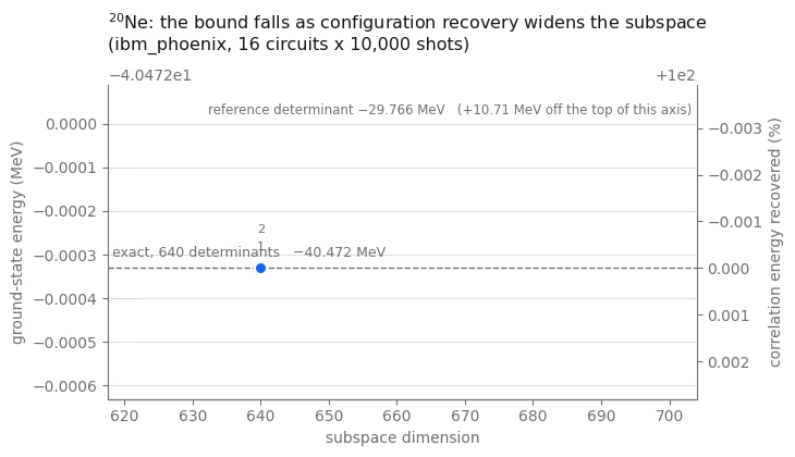
التقطير القطري يعطي حدًا أعلى تغايريًا. نظرًا لأن الفضاء الفرعي لكل تكرار يحتوي على السابق، فإن متتالية الطاقات تتناقص بشكل رتيب، وكل قيمة فيها هي حد أعلى صارم على طاقة الحالة الأساسية الحقيقية، بغض النظر عن الضجيج في العينات التي أنتجتها.

result_sd = recovery_loop(
    inter_sd,
    sp_sd,
    matrix_sd,
    probs_sd,
    occ_sd,
    N_PROTONS,
    N_NEUTRONS,
    max_iterations=4,
    max_dimension=MAX_DIMENSION,
    seed=42,
)

E_SQD_SD = result_sd["energy"]
recovered_sd = 100 * (E_SQD_SD - E_REF_SD) / (E_EXACT_SD - E_REF_SD)

print(f"\nreference determinant   {E_REF_SD:11.6f} MeV")
print(
    f"pooled SQD upper bound         {E_SQD_SD:11.6f} MeV   "
    f"(subspace dimension {len(result_sd['basis'])} of {len(basis_exact_sd)})"
)
print(f"exact diagonalization   {E_EXACT_SD:11.6f} MeV")
print(f"\ncorrelation energy recovered: {recovered_sd:.1f}%")

energies_sd = [h["energy"] for h in result_sd["history"]]
if any(b > a + 1e-9 for a, b in zip(energies_sd, energies_sd[1:])):
    raise AssertionError(
        "the subspaces are not nested; the bound should never rise"
    )
if E_SQD_SD < E_EXACT_SD - 1e-7:
    raise AssertionError(
        f"pooled SQD returned {E_SQD_SD:.6f}, below the exact {E_EXACT_SD:.6f}; "
        "a subspace bound cannot beat the full diagonalization"
    )

iteration 1: 66 proton x 66 neutron halves -> dimension 640, E = -40.472331 MeV
  iteration 2: 66 proton x 66 neutron halves -> dimension 640, E = -40.472331 MeV

reference determinant    -29.765549 MeV
pooled SQD upper bound          -40.472331 MeV   (subspace dimension 640 of 640)
exact diagonalization    -40.472331 MeV

correlation energy recovered: 100.0%

قيّم النتائج

استخدم الفحوصات التالية لتقييم نتائجك على خلفية (backend) من فئة Heron بهذه الإعدادات:

• نجاة اللقطات بناءً على عددي النيوكليونات يقيس نسبة اللقطات التي تحمل عددًا صحيحًا من البروتونات والنيوترونات. يمكن أن تنخفض هذه النسبة مع تزايد حجم السجل. يمكن أن يشير معدل نجاة قريب من الصفر إلى مشكلة في تنفيذ الدارة. تحقق من عمق ISA في الخطوة 2 ومن معايرة الـ Backend، وليس من المعالجة اللاحقة.

• حلقة الاسترجاع ينبغي أن تطبع بُعد فضاء فرعي يبقى ثابتًا أو يتزايد وطاقة تبقى ثابتة أو تنخفض مع كل تكرار. إذا وصل التكرار الأول بالفعل إلى MAX_DIMENSION، فإن الحلّال الكلاسيكي، وليس أخذ العينات، هو القيد المُقيِّد.

• الجزء المسترجَع لـ $^{20}\mathrm{Ne}$ ينبغي أن يكون مرتفعًا، لأن سقف الأنزاتس (ansatz) المحسوب في الخطوة 1 هو فضاء المحددات الكامل المكوّن من 640 محددًا؛ هذا التشغيل هو الحالة التي يكون فيها أخذ العينات، لا قدرة التعبير، هو العائق الوحيد.

• التأكيدان (assertions) في الخلية السابقة يتحققان من الحدود التغايرية. الحد الذي يرتفع يعني أن الفضاءات الفرعية توقفت عن التداخل المتشعب (nested)، والحد الذي يقع تحت الطاقة الدقيقة يعني أن هناك خطأ ما في الهاميلتوني، وليس في العتاد.

بشكل مخالف للحدس، يمكن لخلفية (backend) أكثر ضجيجًا أن تعطي حدًا أفضل قليلاً من خلفية نظيفة، لأن الأخطاء تنتج أنصاف تكوينات صالحة لم يكن ليأخذ الدارة المثالية عينات منها أبدًا، وتوسيع فضاء فرعي تغايري لا يمكن أن يرفع قيمته الذاتية الدنيا. يمكن للمحاكاة المشوبة بالضجيج أن تُظهر التأثير نفسه؛ يُظهره هذا الدرس التعليمي باستخدام عينات من عتاد حقيقي.

# IBM Carbon palette: Blue 60 and Blue 80 for data, Gray 100/70/30 for ink and rules
SURFACE, INK, MUTED, RULE = "#ffffff", "#161616", "#6f6f6f", "#c6c6c6"
SERIES, DEEP, PURPLE = "#0f62fe", "#002d9c", "#6929c4"

def convergence_plot(
    history, e_ref, e_exact, title, colour=SERIES, full_dim=None
):
    """Energy against subspace dimension, scaled to the data rather than to the full window.

    A good run lands within a fraction of a percent of the exact answer, so an axis spanning
    reference-to-exact would squash every point onto one line.  The axis is therefore scaled to
    the data (plus the exact line, when there is one), and the right-hand axis carries the
    fraction of the correlation energy so the absolute and relative readings sit side by side.
    """
    dimensions = [h["dimension"] for h in history]
    energies = [h["energy"] for h in history]

    fig, ax = plt.subplots(figsize=(7.4, 4.3), facecolor=SURFACE)
    ax.set_facecolor(SURFACE)
    ax.plot(
        dimensions,
        energies,
        "-o",
        color=colour,
        linewidth=2,
        markersize=8,
        markeredgecolor=SURFACE,
        markeredgewidth=1.5,
        zorder=3,
    )
    stacked = {}
    for h in history:
        # a converged loop repeats the same point; stack the labels so they do not overprint
        key = (round(h["dimension"]), round(h["energy"], 9))
        offset = 12 + 11 * stacked.get(key, 0)
        stacked[key] = stacked.get(key, 0) + 1
        ax.annotate(
            str(h["iteration"]),
            xy=(h["dimension"], h["energy"]),
            xytext=(0, offset),
            textcoords="offset points",
            ha="center",
            fontsize=8,
            color=MUTED,
        )

    span = (max(dimensions) - min(dimensions)) or max(1, max(dimensions) // 4)
    x_left, x_right = (
        min(dimensions) - 0.14 * span,
        max(dimensions) + 0.40 * span,
    )
    ax.set_xlim(x_left, x_right)

    floor = min(energies) if e_exact is None else min(min(energies), e_exact)
    height = max(max(energies) - floor, 1e-3)
    ax.set_ylim(floor - 0.30 * height, max(energies) + 0.42 * height)

    if e_exact is not None:
        ax.axhline(
            e_exact, color=MUTED, linestyle="--", linewidth=1, zorder=1
        )
        label = "exact" + (f", {full_dim:,} determinants" if full_dim else "")
        ax.annotate(
            f"{label}   {e_exact:.3f} MeV".replace("-", "\u2212"),
            xy=(x_left, e_exact),
            xytext=(3, 5),
            textcoords="offset points",
            ha="left",
            va="bottom",
            color=MUTED,
            fontsize=9,
        )

    # the reference determinant is far off this scale; state it rather than plotting it
    ax.annotate(
        f"reference determinant {e_ref:.3f} MeV".replace("-", "\u2212")
        + f"   ({e_ref - max(energies):+.2f} MeV off the top of this axis)".replace(
            "-", "\u2212"
        ),
        xy=(x_right, max(energies) + 0.42 * height),
        xytext=(-3, -12),
        textcoords="offset points",
        ha="right",
        va="top",
        color=MUTED,
        fontsize=8.5,
    )

    if e_exact is not None and abs(e_exact - e_ref) > 1e-9:
        right = ax.twinx()
        low, high = ax.get_ylim()

        def to_percent(e):
            return 100 * (e - e_ref) / (e_exact - e_ref)

        right.set_ylim(to_percent(low), to_percent(high))
        right.set_ylabel("correlation energy recovered (%)", color=MUTED)
        right.tick_params(colors=MUTED)
        for side in ("top", "left"):
            right.spines[side].set_visible(False)
        right.spines["right"].set_color(MUTED)
        right.spines["bottom"].set_color(MUTED)

    ax.set_xlabel("subspace dimension", color=MUTED)
    ax.set_ylabel("ground-state energy (MeV)", color=MUTED)
    ax.set_title(title, color=INK, fontsize=11.5, loc="left", pad=12)
    ax.grid(axis="y", color=RULE, alpha=0.55)
    ax.tick_params(colors=MUTED)
    for side in ("top", "right"):
        ax.spines[side].set_visible(False)
    for side in ("bottom", "left"):
        ax.spines[side].set_color(MUTED)
    fig.tight_layout()
    return fig

convergence_plot(
    result_sd["history"],
    E_REF_SD,
    E_EXACT_SD,
    f"$^{{20}}$Ne: the bound falls as configuration recovery widens the subspace\n"
    f"({backend.name}, {N_CIRCUITS} circuits x {SHOTS:,} shots)",
    full_dim=len(basis_exact_sd),
)
plt.show()

مثال على العتاد بمقياس كبير

التوسع في المقياس لا يُغيّر سوى المدخلات، لذا فالخطوة التالية هي دمج المراحل الأربع في دالة واحدة وتشغيلها مرتين، كلتاهما على سجل من 40 كيوبت في قشرة $pf$ فوق نواة $^{40}\mathrm{Ca}$ مع تفاعل GXPF1 [3].

يوضح التشغيلان جانبين مختلفين من التوسع في المقياس:

• $^{44}\mathrm{Ti}$، ببروتونَي تكافؤ ونيوترونَي تكافؤ، له أساس مكوّن من 4000 محدِّد. السجل مكوّن من 40 كيوبت، لكن المسألة لا تزال صغيرة بما يكفي للتقطير القطري الدقيق على حاسوب محمول، لذا يمكنك مقارنة نتيجة العتاد بمرجع دقيق بعد زيادة حجم السجل.

• $^{48}\mathrm{Cr}$، بأربعة بروتونات تكافؤ وأربعة نيوترونات تكافؤ، له 1,963,461 محدِّدًا مسموحًا به تماثليًا في نفس الـ 40 كيوبت. لا يستطيع الحلّال الكثيف في هذا الدرس التعليمي تقطير ذلك الفضاء الكامل، لذا يُعيد التشغيل حدًا أعلى صارمًا والمحدِّد المرجعي الذي يُحسّن عليه.

راقب كميتين عبر التشغيلين. ينكمش الجزء من التجمّع (pool) الذي يتسع داخل ميزانية البوابات الثابتة مع نمو التجمّع، وتُبلغ pack_ensemble عن مقدار ما تم تضمينه. يتوقف الفضاء الفرعي عن أن يكون مقيَّدًا بأخذ العينات ويصبح مقيَّدًا بـ MAX_DIMENSION، أكبر مصفوفة يبنيها الحلّال الكلاسيكي الكثيف هنا. بهذا المقياس، سيستخدم حساب إنتاجي حلّال تفاعل التكوين المُختار (selected-CI).

دمج الخطوات 1-4

تستدعي الدالة التالية نفس المراحل الواردة في الدليل الإرشادي، وبنفس الترتيب.

def sqd_run(snt_file, n_protons, n_neutrons, name, exact=True):
    """The whole workflow for one nucleus.  Returns a record of every stage."""
    # -------------------------Step 1-------------------------
    ms = read_snt(DATA / snt_file, n_protons, n_neutrons)
    sp = m_scheme_states(ms)
    inter = Interaction(ms, sp)
    if sum(1 for s in sp if s.tz == -1) * 2 != len(sp):
        raise ValueError(
            f"{name}: post-selection needs equal proton and neutron state counts"
        )
    reference = reference_determinant(sp, inter, n_protons, n_neutrons)
    e_ref = matrix_element(inter, reference, reference)

    raw = excitation_pool(sp, reference)
    ranked = rank_pool(
        inter, reference, [op for op in raw if conserves_symmetry(sp, op)]
    )
    print(
        f"{name}: {len(sp)} qubits, {n_protons}p + {n_neutrons}n, A = {ms.mass_number}"
    )
    print(
        f"  2p2h pool {len(raw)} raw -> {len(ranked)} symmetry-allowed; "
        f"reference energy {e_ref:.6f} MeV"
    )

    # -------------------------Step 2-------------------------
    costs = excitation_costs(len(sp), ranked, costing_manager)
    circuits, bins, isa = pack_to_budget(
        len(sp),
        reference,
        ranked,
        costs,
        DEPTH_BUDGET,
        N_CIRCUITS,
        pass_manager,
    )
    packed = sum(len(b) for b in bins)
    worst = max(two_qubit_depth(c) for c in isa)
    worst_count = max(two_qubit_count(c) for c in isa)
    print(
        f"  packed {packed} of {len(ranked)} excitations; worst circuit two-qubit depth "
        f"{worst}, {worst_count} two-qubit gates"
    )

    # -------------------------Step 3-------------------------
    # a unique tag per run, so the jobs are findable later
    bit_arrays = sample(isa, SHOTS, JOB_TAGS + [name])
    matrix, probabilities, shots = pool_samples(bit_arrays, sp)
    survival = float(
        probabilities[
            (matrix[:, len(sp) // 2 :].sum(axis=1) == n_protons)
            & (matrix[:, : len(sp) // 2].sum(axis=1) == n_neutrons)
        ].sum()
    )
    print(
        f"  {shots:,} shots -> {len(matrix):,} distinct bitstrings, "
        f"{survival:.1%} of shots with the right nucleon numbers"
    )
    if survival == 0.0:
        raise RuntimeError(
            f"{name}: no shot carried the right nucleon numbers"
        )

    # -------------------------Step 4-------------------------
    result = recovery_loop(
        inter,
        sp,
        matrix,
        probabilities,
        reference,
        n_protons,
        n_neutrons,
        max_iterations=4,
        max_dimension=MAX_DIMENSION,
        seed=42,
    )
    energy = result["energy"]

    full_dim = count_basis(sp, n_protons, n_neutrons)  # cheap, even when huge
    e_exact = None
    if exact:
        full = full_basis(sp, n_protons, n_neutrons)
        if len(full) != full_dim:
            raise AssertionError(
                f"{name}: counted {full_dim} determinants but enumerated "
                f"{len(full)}"
            )
        e_exact, _ = ground_state(inter, full)

    print(f"  reference {e_ref:11.6f} MeV     pooled SQD {energy:11.6f} MeV")
    if e_exact is not None:
        print(
            f"  exact     {e_exact:11.6f} MeV  (dimension {full_dim})  ->  "
            f"{100 * (energy - e_ref) / (e_exact - e_ref):.1f}% of the correlation energy"
        )
        if energy < e_exact - 1e-7:
            raise AssertionError(
                f"{name}: pooled SQD bound is below the exact energy"
            )
    else:
        print(
            f"  no exact reference: the symmetry-allowed basis is {full_dim:,} determinants"
        )
        print(
            f"  the bound captures {energy - e_ref:.6f} MeV of correlation energy"
        )
    print()

    return dict(
        name=name,
        qubits=len(sp),
        pool=len(ranked),
        packed=packed,
        two_qubit=worst,
        two_qubit_gates=worst_count,
        shots=shots,
        distinct=len(matrix),
        survival=survival,
        dimension=len(result["basis"]),
        full_dim=full_dim,
        e_ref=e_ref,
        e_sqd=energy,
        e_exact=e_exact,
        history=result["history"],
        # the subspace and its eigenvector cannot be reconstructed from the summary --
        # they depend on the sampled shots -- so keep them for the scaling analysis
        interaction=inter,
        states=sp,
        reference=reference,
        ranked=ranked,
        basis=result["basis"],
        vector=result["vector"],
    )

pretty = {"20Ne": "$^{20}$Ne", "44Ti": "$^{44}$Ti", "48Cr": "$^{48}$Cr"}

small_scale = dict(
    name="20Ne",
    qubits=len(sp_sd),
    pool=len(ranked_sd),
    packed=PACKED_SD,
    two_qubit=worst_sd,
    two_qubit_gates=worst_count_sd,
    shots=shots_sd,
    distinct=len(matrix_sd),
    survival=shot_survival_sd,
    dimension=len(result_sd["basis"]),
    full_dim=len(basis_exact_sd),
    e_ref=E_REF_SD,
    e_sqd=E_SQD_SD,
    e_exact=E_EXACT_SD,
    history=result_sd["history"],
    interaction=inter_sd,
    states=sp_sd,
    reference=occ_sd,
    ranked=ranked_sd,
    basis=result_sd["basis"],
    vector=result_sd["vector"],
)

$^{44}\mathrm{Ti}$: نفس سير العمل على سجل من 40 كيوبت

تحتوي قشرة $pf$ فوق $^{40}\mathrm{Ca}$ على أربعة مدارات لكل نوع و20 حالة فرعية مغناطيسية لكل منها، لذا فالسجل مكوّن من 40 كيوبت. يكوّن بروتونا تكافؤ ونيوترونا تكافؤ $^{44}\mathrm{Ti}$، بـ 4000 محدِّد مسموح به تماثليًا — أي حوالي ستة أضعاف أساس $^{20}\mathrm{Ne}$، باستخدام 40 كيوبت بدلاً من 24.

هذا هو الأكبر من بين المثالين اللذين يستطيع الدفتر حلّهما بدقة، لذا يمكنك مقارنة نتيجة العتاد بمرجع دقيق.

large_scale_verified = sqd_run("gxpf1.snt", 2, 2, "44Ti", exact=True)

44Ti: 40 qubits, 2p + 2n, A = 44
  2p2h pool 1602 raw -> 174 symmetry-allowed; reference energy -44.309387 MeV
  packed 96 of 174 excitations; worst circuit two-qubit depth 272, 285 two-qubit gates
job dap31a02fm4c73f67dp0: 16 circuits x 10,000 shots on ibm_phoenix
  160,000 shots -> 48,170 distinct bitstrings, 18.6% of shots with the right nucleon numbers
  iteration 1: 187 proton x 189 neutron halves -> dimension 3891, E = -47.849086 MeV
  iteration 2: 190 proton x 190 neutron halves -> dimension 4000, E = -47.876666 MeV
  iteration 3: 190 proton x 190 neutron halves -> dimension 4000, E = -47.876666 MeV
  reference  -44.309387 MeV     pooled SQD  -47.876666 MeV
  exact      -47.876666 MeV  (dimension 4000)  ->  100.0% of the correlation energy

$^{48}\mathrm{Cr}$: تجاوز قدرة الدرس التعليمي على التقطير القطري الدقيق

إضافة بروتونين ونيوترونين تستخدم نفس السجل المكوّن من 40 كيوبت (4, 4 لـ $^{48}\mathrm{Cr}$) وتزيد حجم الأساس بعامل يبلغ نحو 491، ليصل إلى 1,963,461 محدِّدًا مسموحًا به تماثليًا. تلك المصفوفة أبعد بكثير من أي شيء سيبنيه هذا الدرس التعليمي، لذا exact=False: فلا توجد طاقة مرجعية دقيقة، بل فقط الحد التغايري والمحدِّد المرجعي الذي يُحسّن عليه.

يتغيّر شيئان عند هذا المقياس، وكلاهما ظاهر في المُخرَج المطبوع. يكبر التجمّع (pool) ليصل إلى عدة مئات من الإثارات المسموح بها، لذا فميزانية البوابات الثابتة تغطي الآن أقلية منه بدلاً من كله. كذلك، فإن الفضاء الفرعي للنواتج الذي تُمثّله العينات أكبر من MAX_DIMENSION، لذا يقوم الحلّال الكثيف باقتطاعه حسب الوزن المأخوذ بالعينة. يظل الحد صارمًا لكنه قد يكون أقل دقة من حد محسوب من جميع التكوينات المأخوذة بالعينة. سيحتفظ الحساب الإنتاجي بالعينات ويستخدم حلّالاً يدعم فضاءً فرعيًا أكبر.

large_scale_unverified = sqd_run("gxpf1.snt", 4, 4, "48Cr", exact=False)

48Cr: 40 qubits, 4p + 4n, A = 48
  2p2h pool 5536 raw -> 582 symmetry-allowed; reference energy -93.041237 MeV
  packed 96 of 582 excitations; worst circuit two-qubit depth 224, 279 two-qubit gates
job dap32a02fm4c73f67eog: 16 circuits x 10,000 shots on ibm_phoenix
  160,000 shots -> 55,436 distinct bitstrings, 18.6% of shots with the right nucleon numbers
  iteration 1: 223 proton x 223 neutron halves -> dimension 3977, E = -96.481598 MeV
  iteration 2: 223 proton x 223 neutron halves -> dimension 3977, E = -96.481598 MeV
  reference  -93.041237 MeV     pooled SQD  -96.481598 MeV
  no exact reference: the symmetry-allowed basis is 1,963,461 determinants
  the bound captures -3.440361 MeV of correlation energy

قيّم نتيجة بدون مرجع دقيق

لا يمتلك تشغيل $^{48}\mathrm{Cr}$ مرجعًا دقيقًا ضمن هذا الدرس التعليمي. استخدم العينات الموجودة لتقييم التقارب والمقارنة بخط الأساس الكلاسيكي للاختيار، دون الحاجة إلى وقت إضافي على الـ QPU أو تقطير قطري للفضاء الكامل.

هل تحقق التقارب؟ إعادة ترتيب المحدِّدات المحتفَظ بها حسب وزنها في المتجه الذاتي المتقارب تجعل الفضاءات الفرعية متداخلة (nested)، بحيث أن تقطير الكتلة الرئيسية $d \times d$ لسلّم من قيم $d$ يرسم مسار انخفاض الحد عبر عقدين من أحجام الفضاء الفرعي. إذا كان لا يزال ينخفض بشدة عند أكبر $d$، فإن سقف بُعد الحلّال الكلاسيكي هو القيد المُقيِّد وMAX_DIMENSION هي المعامل الواجب زيادته. أما إذا تسطّح، فإن إضافة المزيد من المحدِّدات المحتفَظ بها تقدّم تحسنًا ضئيلًا؛ وقد يتطلب مزيد من التقدم أخذ عينات لتكوينات إضافية. يُبنى الهاميلتوني مرة واحدة بالحجم الكامل وكل درجة في السلّم هي كتلة رئيسية منه، لذا فإن المسح بأكمله يكلّف بناء مصفوفة واحدة بدلاً من بناء واحدة لكل درجة.

كيف يُقارَن أخذ العينات الكمومي باختيار كلاسيكي؟ قارن بفضاء فرعي من نفس الحجم يُختار بواسطة إجراء الاختيار الكلاسيكي: خذ التجمّع مرتبًا بنظرية الاضطراب حسب ترتيب الدرجة، ووسّع فضاء النواتج الفرعي إلى نفس البُعد، وقطّر ذلك بدلاً منه. كلا المنحنيين حدود عليا صارمة على نفس الهاميلتوني، لذا فأيهما يقع أدنى عند بُعد مساوٍ يكون قد اختار المحدِّدات الأفضل. تحدد هذه المقارنة ما إذا كان أخذ العينات على العتاد يحسّن تقدير الطاقة مقارنةً بخط الأساس الكلاسيكي هذا.

لم يُختَر هذا الفضاء الفرعي من أجل الحالات المثارة. يوجّه استرجاع التكوين الفضاء الفرعي باستخدام إشغالات الحالة الأساسية، لذا فإن القيم الذاتية الأعلى أبعد كثيرًا عن التقارب من أدناها، وتأتي طاقة الإثارة الأولى أعلى بكثير من قيمة $2^+$ المقاسة. يتطلب الوصول السليم إلى الحالات المثارة فضاءً فرعيًا مُختارًا من أجلها.

def subspace_scaling(
    inter, basis, vector, points=18, smallest=32, largest=None
):
    """Nested Rayleigh-Ritz sweep: the lowest eigenvalue of the leading d x d block, for a ladder of d.

    Reordering the basis by descending weight in the converged eigenvector makes every subspace in
    the ladder a subset of the next, so the energies fall monotonically and each one is a valid
    variational bound.  H is built once at full size; each rung is a principal block.
    """
    order = np.argsort(-(np.abs(vector) ** 2))
    ordered = [basis[i] for i in order]
    weights = (np.abs(vector) ** 2)[order]
    if (
        largest is not None
    ):  # cap the ladder so two subspaces end at a common dimension
        ordered, weights = ordered[:largest], weights[:largest]
    H = subspace_hamiltonian(inter, ordered)
    dimensions = np.unique(
        np.geomspace(smallest, len(ordered), points).astype(int)
    )
    rows = [
        (
            int(d),
            float(
                eigh(H[:d, :d], eigvals_only=True, subset_by_index=[0, 0])[0]
            ),
        )
        for d in dimensions
    ]
    return rows, np.cumsum(weights)

def classical_selection(
    inter, sp, reference, ranked, target, n_protons, n_neutrons
):
    """The subspace classical perturbative ranking would pick, grown to `target` dimension.

    Same product construction as the sampled subspace, and the same truncation discipline -- half
    configurations are offered to `grow_subspace` in order of importance and it takes as many as
    fit.  The only difference from the sampled path is where the ordering comes from: PT2 score
    here, measured sampling weight there.  So the comparison isolates *which determinants got
    chosen* and nothing else.

    Truncating by any other rule would not be a fair baseline.  Slicing an arbitrarily ordered
    list, for instance, keeps determinants by accident rather than by importance and makes the
    classical subspace look worse than classical selection really is.
    """
    p_ref = tuple(i for i in reference if sp[i].tz == -1)
    n_ref = tuple(i for i in reference if sp[i].tz == +1)
    reached = {reference}
    proton_order, neutron_order = [p_ref], [n_ref]
    seen_p, seen_n = {p_ref}, {n_ref}
    product_budget = 4 * target

    for op, _, _ in ranked:  # ranked is already in descending PT2 score
        h1, h2, v1, v2 = op
        fresh = {
            tuple(sorted(set(d) - {h1, h2} | {v1, v2}))
            for d in reached
            if {h1, h2} <= set(d) and not {v1, v2} & set(d)
        }
        reached |= fresh
        for det in fresh:  # first appearance fixes a half's rank
            half_p = tuple(i for i in det if sp[i].tz == -1)
            half_n = tuple(i for i in det if sp[i].tz == +1)
            if half_p not in seen_p:
                seen_p.add(half_p)
                proton_order.append(half_p)
            if half_n not in seen_n:
                seen_n.add(half_n)
                neutron_order.append(half_n)
        if len(proton_order) * len(neutron_order) > product_budget:
            # Half-configuration products over-count the subspace, because only the
            # symmetry-allowed ones survive `product_subspace`.  Stopping on the product
            # count alone can therefore leave the basis far short of `target`, so check
            # the dimension actually realized and widen the budget if it falls short.
            trial, _, _ = grow_subspace(
                sp,
                [p_ref],
                [n_ref],
                proton_order,
                neutron_order,
                n_protons,
                n_neutrons,
                max_dimension=target,
            )
            if len(trial) >= target:
                break
            product_budget *= 2

    basis, _, _ = grow_subspace(
        sp,
        [p_ref],
        [n_ref],
        proton_order,
        neutron_order,
        n_protons,
        n_neutrons,
        max_dimension=target,
    )
    return basis

run = large_scale_unverified
if "basis" not in run:
    raise RuntimeError(
        "this cell needs the subspace and eigenvector that sqd_run now returns; "
        "re-run the sqd_run definition and the 48Cr cell"
    )

print(
    f"{run['name']}: sweeping nested subspaces of the sampled basis "
    f"(dimension {run['dimension']})"
)
sampled_rows, cumulative = subspace_scaling(
    run["interaction"], run["basis"], run["vector"]
)

print(
    f"{run['name']}: building the classically selected subspace at the same dimension"
)
classical_basis = classical_selection(
    run["interaction"],
    run["states"],
    run["reference"],
    run["ranked"],
    run["dimension"],
    4,
    4,
)
# Both subspaces must be scored at the same dimension.  Symmetry filtering can still leave
# the classical construction short of the target when the ranked pool runs out, so take the
# dimension both actually reach, cap both ladders there, and verify they agree.
common_dim = min(sampled_rows[-1][0], len(classical_basis))
if common_dim < sampled_rows[-1][0]:
    sampled_rows, _ = subspace_scaling(
        run["interaction"], run["basis"], run["vector"], largest=common_dim
    )
classical_rows, _ = subspace_scaling(
    run["interaction"],
    classical_basis,
    ground_state(run["interaction"], classical_basis)[1],
    largest=common_dim,
)
if sampled_rows[-1][0] != classical_rows[-1][0]:
    raise RuntimeError(
        f"comparison dimensions differ: sampled {sampled_rows[-1][0]}, "
        f"classical {classical_rows[-1][0]}"
    )

advantage = sampled_rows[-1][1] - classical_rows[-1][1]
direction = "lower" if advantage < 0 else "higher"
verdict = "beats" if advantage < 0 else "does not beat"
descent = next(
    e for d, e in reversed(sampled_rows) if d <= sampled_rows[-1][0] / 2
)
for fraction in (0.90, 0.99):
    count = int(np.searchsorted(cumulative, fraction) + 1)
    print(
        f"  {fraction:.0%} of the eigenvector norm sits on {count} determinants "
        f"({count / run['full_dim']:.1e} of the {run['full_dim']:,}-determinant space)"
    )
print(
    f"  bound still falling {1000 * (sampled_rows[-1][1] - descent):+.1f} keV "
    f"over the last doubling of dimension"
)
print(
    f"  sampled {sampled_rows[-1][1]:.6f} MeV vs classically selected "
    f"{classical_rows[-1][1]:.6f} MeV at a verified common dimension of "
    f"{classical_rows[-1][0]:,}"
)
print(
    f"  -> the sampled subspace is {abs(advantage) * 1000:.0f} keV {direction}"
)

48Cr: sweeping nested subspaces of the sampled basis (dimension 3977)
48Cr: building the classically selected subspace at the same dimension
  90% of the eigenvector norm sits on 107 determinants (5.4e-05 of the 1,963,461-determinant space)
  99% of the eigenvector norm sits on 593 determinants (3.0e-04 of the 1,963,461-determinant space)
  bound still falling -15.6 keV over the last doubling of dimension
  sampled -96.481598 MeV vs classically selected -95.314510 MeV at a verified common dimension of 3,957
  -> the sampled subspace is 1167 keV lower

fig, axes = plt.subplots(1, 2, figsize=(11.2, 4.0), facecolor=SURFACE)

# left: two nested convergence curves on the same axes
ax = axes[0]
ax.set_facecolor(SURFACE)
ax.plot(
    [d for d, _ in sampled_rows],
    [e for _, e in sampled_rows],
    "-o",
    color=SERIES,
    linewidth=2,
    markersize=5,
    markeredgecolor=SURFACE,
    markeredgewidth=1,
    zorder=4,
    label="sampled on the QPU",
)
ax.plot(
    [d for d, _ in classical_rows],
    [e for _, e in classical_rows],
    "--s",
    color=MUTED,
    linewidth=1.6,
    markersize=4,
    markeredgecolor=SURFACE,
    markeredgewidth=1,
    zorder=3,
    label="classically selected, same size",
)
ax.axhline(run["e_ref"], color=RULE, linestyle=":", linewidth=1.2, zorder=1)
ax.annotate(
    f"reference determinant {run['e_ref']:.2f} MeV".replace("-", "\u2212"),
    xy=(sampled_rows[-1][0], run["e_ref"]),
    xytext=(-2, 4),
    textcoords="offset points",
    ha="right",
    va="bottom",
    color=MUTED,
    fontsize=8,
)

# mark the gap between the two curves at the largest dimension, not either curve alone
edge = sampled_rows[-1][0]
ax.plot(
    [edge, edge],
    [classical_rows[-1][1], sampled_rows[-1][1]],
    "-",
    color=SERIES,
    linewidth=1.0,
    alpha=0.7,
    zorder=2,
)
ax.annotate(
    f"{abs(advantage) * 1000:.0f} keV {direction}\nat equal dimension",
    xy=(edge, 0.5 * (classical_rows[-1][1] + sampled_rows[-1][1])),
    xytext=(-8, 0),
    textcoords="offset points",
    ha="right",
    va="center",
    color=SERIES,
    fontsize=8.5,
)

ax.set_xscale("log")
ax.set_xlim(sampled_rows[0][0] * 0.75, edge * 1.5)
ax.set_xlabel("subspace dimension", color=MUTED)
ax.set_ylabel("variational upper bound (MeV)", color=MUTED)
ax.set_title(
    f"{pretty[run['name']]}: the bound, and the subspace it {verdict}",
    color=INK,
    fontsize=11,
    loc="left",
    pad=10,
)
legend = ax.legend(frameon=False, fontsize=8.5, loc="lower left")
for text in legend.get_texts():
    text.set_color(MUTED)

# right: why a few thousand determinants can bound two million
ax = axes[1]
ax.set_facecolor(SURFACE)
ranks = np.arange(1, len(cumulative) + 1)
ax.plot(ranks, 100 * cumulative, "-", color=DEEP, linewidth=2, zorder=3)
for fraction, style, label_y in ((0.90, ":", 46), (0.99, "--", 24)):
    count = int(np.searchsorted(cumulative, fraction) + 1)
    ax.axvline(count, color=MUTED, linestyle=style, linewidth=1, zorder=1)
    ax.annotate(
        f"{fraction:.0%} of the norm\non {count} determinants",
        xy=(count, label_y),
        xytext=(7, 0),
        textcoords="offset points",
        ha="left",
        va="center",
        color=MUTED,
        fontsize=8.5,
    )
ax.set_xscale("log")
ax.set_xlim(0.8, len(cumulative) * 2.6)
ax.set_ylim(0, 104)
ax.set_xlabel("determinants, ordered by weight", color=MUTED)
ax.set_ylabel("cumulative share of the eigenvector (%)", color=MUTED)
ax.set_title(
    f"Sparsity: {run['full_dim']:,} determinants in the sector",
    color=INK,
    fontsize=11,
    loc="left",
    pad=10,
)

for ax in axes:
    ax.grid(axis="y", color=RULE, alpha=0.55)
    ax.tick_params(colors=MUTED, labelsize=8.5)
    for side in ("top", "right"):
        ax.spines[side].set_visible(False)
    for side in ("bottom", "left"):
        ax.spines[side].set_color(MUTED)
fig.tight_layout()
plt.show()

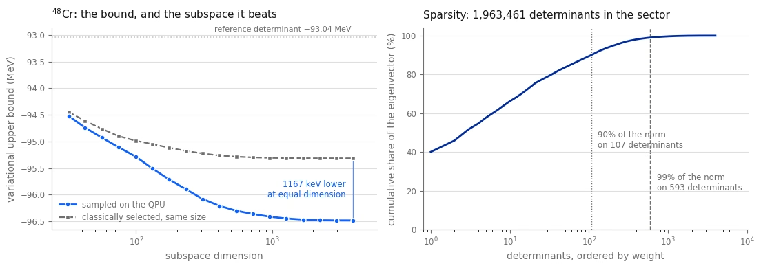
قارن التشغيلات الثلاثة

الطاقات المطلقة غير قابلة للمقارنة بين أنوية وتفاعلات مختلفة، لذا ركّز على نسبة طاقة الترابط المسترجَعة عبر التشغيلات، حيثما يتوفر مرجع دقيق. قارن أيضًا عمق الدارة ونسبة اللقطات المُهملة.

runs = [small_scale, large_scale_verified, large_scale_unverified]

print(
    f"{'run':>6}  {'qubits':>6}  {'pool':>9}  {'2q depth':>8}  {'2q gates':>8}  "
    f"{'shots kept':>10}  {'dim':>6}  {'of':>9}  {'% corr':>7}"
)
for r in runs:
    fraction = (
        "--"
        if r["e_exact"] is None
        else f"{100 * (r['e_sqd'] - r['e_ref']) / (r['e_exact'] - r['e_ref']):.1f}%"
    )
    coverage = "{}/{}".format(r["packed"], r["pool"])
    print(
        f"{r['name']:>6}  {r['qubits']:>6}  {coverage:>9}  "
        f"{r['two_qubit']:>8}  {r['two_qubit_gates']:>8}  {r['survival']:>9.1%}  "
        f"{r['dimension']:>6}  {(r['full_dim'] or 0):>9,}  {fraction:>7}"
    )

print()
for r in runs:
    exact = (
        f"exact {r['e_exact']:11.6f}"
        if r["e_exact"] is not None
        else "exact  unavailable"
    )
    print(
        f"{r['name']:>6}   reference {r['e_ref']:11.6f}   pooled SQD {r['e_sqd']:11.6f}   {exact} MeV"
    )

run  qubits       pool  2q depth  2q gates  shots kept     dim         of   % corr
  20Ne      24      78/78       228       234      31.5%     640        640   100.0%
  44Ti      40     96/174       272       285      18.6%    4000      4,000   100.0%
  48Cr      40     96/582       224       279      18.6%    3977  1,963,461       --

  20Ne   reference  -29.765549   pooled SQD  -40.472331   exact  -40.472331 MeV
  44Ti   reference  -44.309387   pooled SQD  -47.876666   exact  -47.876666 MeV
  48Cr   reference  -93.041237   pooled SQD  -96.481598   exact  unavailable MeV

# Left: how much of the correlation energy was recovered, where the exact answer is known.
# Right: the bound itself for the run that has nothing to score against.
scored = [r for r in runs if r["e_exact"] is not None]

fig, ax = plt.subplots(figsize=(6.4, 3.9), facecolor=SURFACE)
ax.set_facecolor(SURFACE)
labels = [
    f"{pretty[r['name']]}\n{r['qubits']} qubits\n{r['full_dim']:,} determinants"
    for r in scored
]
fractions = [
    100 * (r["e_sqd"] - r["e_ref"]) / (r["e_exact"] - r["e_ref"])
    for r in scored
]
shades = [SERIES, DEEP, PURPLE]
bars = ax.bar(
    labels, fractions, width=0.46, color=shades[: len(scored)], zorder=3
)
for bar, fraction, r in zip(bars, fractions, scored):
    ax.annotate(
        f"{fraction:.1f}%",
        xy=(bar.get_x() + bar.get_width() / 2, fraction),
        xytext=(0, 5),
        textcoords="offset points",
        ha="center",
        va="bottom",
        color=INK,
        fontsize=10,
    )
    ax.annotate(
        f"dim {r['dimension']:,}",
        xy=(bar.get_x() + bar.get_width() / 2, 3),
        ha="center",
        va="bottom",
        color=SURFACE,
        fontsize=8.5,
    )
ax.axhline(100, color=MUTED, linestyle="--", linewidth=1, zorder=1)
ax.annotate(
    "exact diagonalization",
    xy=(-0.45, 100),
    xytext=(0, 4),
    textcoords="offset points",
    ha="left",
    va="bottom",
    color=MUTED,
    fontsize=8.5,
)
ax.set_ylim(0, 118)
ax.set_ylabel("correlation energy recovered (%)", color=MUTED)
ax.set_title(
    f"Where the exact answer is known ({backend.name})",
    color=INK,
    fontsize=11,
    loc="left",
    pad=10,
)
ax.grid(axis="y", color=RULE, alpha=0.55)
ax.tick_params(colors=MUTED, labelsize=8.5)
for side in ("top", "right"):
    ax.spines[side].set_visible(False)
for side in ("bottom", "left"):
    ax.spines[side].set_color(MUTED)
fig.tight_layout()
plt.show()

# the same convergence view as the walkthrough, for the run with no exact reference
convergence_plot(
    large_scale_unverified["history"],
    large_scale_unverified["e_ref"],
    None,
    f"{pretty[large_scale_unverified['name']]}: "
    f"{large_scale_unverified['full_dim']:,} determinants, no exact answer to score against\n"
    f"({backend.name}, {N_CIRCUITS} circuits x {SHOTS:,} shots)",
    colour=DEEP,
)
plt.show()

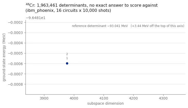
ملخص

سار سير عمل واحد، دون تغيير باستثناء مدخلاته، على QPU بثلاثة أحجام للمسألة: مسألة من 24 كيوبت يمكنك التحقق منها بدقة، ومسألة من 40 كيوبت لا يزال بإمكانك التحقق منها بدقة، ومسألة من 40 كيوبت بما يقارب مليوني حالة أساس تتجاوز قدرة هذا الدرس التعليمي على التقطير القطري الدقيق.

توضح التشغيلات الثلاثة النقاط التالية:

• لا يتعيّن على الخطوة الكمومية سوى اقتراح المحدِّدات. الدارة ثابتة، مُهيّأة من نظرية الاضطراب من الرتبة الثانية، ولا يتم تحسينها أبدًا. لا يحتاج أي جزء من سير العمل إلى أن تكون سعاتها دقيقة، بل فقط أن يكون مجالها (support) مفيدًا. يعطي التقطير القطري الكلاسيكي في الفضاء الفرعي المُختار حدًا أعلى تغايريًا، رغم أن الحد يتفاوت مع التكوينات المأخوذة بالعينة.

• إثارات الكيوبت تقلل عمق الدارة. نظرًا لأن المجال (support) وحده هو المهم، يمكن استبدال كتل الإثارة الفرميونية بإثارات كيوبت، لا تزداد تكلفتها مع المسافة بين المدارات التي تربطها. قاست الخطوة 2 التوفير على الـ Backend الفعلي، وهو الفارق بين دارة تتسع بارتياح داخل زمن الترابط (coherence) وأخرى لا تتسع.

• استرجاع التكوين يعيد استخدام العينات المشوبة بالضجيج. كل لقطة بعدد بروتونات أو نيوترونات خاطئ يتم إصلاحها مقابل تقدير الإشغال الحالي بدلاً من تجاهلها، ويمكن لكل نصف تكوين تم إصلاحه أن يضيف تكوينات إلى الفضاء الفرعي. توسيع الفضاء الفرعي التغايري لا يمكن أن يرفع قيمته الذاتية الدنيا. يُظهر هذا الدرس التعليمي استرجاع التكوين باستخدام عينات من العتاد.

• القيد المُقيِّد يتنقل مع تغير المقياس. عند 24 كيوبت كان بإمكان الأنزاتس (ansatz) الوصول إلى الإجابة الدقيقة، وكان أخذ العينات وحده هو العائق. عند 40 كيوبت بأربعة نيوكليونات تكافؤ لكل نوع، تغطي ميزانية البوابات أقلية من التجمّع ويحدّ الحلّال الكلاسيكي الكثيف من الفضاء الفرعي. معرفة أيّ من العوامل الثلاثة يقيّدك هي المهارة العملية التي يعلّمها سير العمل هذا.

الخطوات التالية

توصيات

استكشف هذه الموارد ذات الصلة:

• التقطير القطري الكمومي المعتمد على العينات لهاميلتوني كيميائي: نفس الخوارزمية مُطبّقة على البنية الإلكترونية، باستخدام حلّال selected-CI الخاص بإضافة SQD.

• توثيق إضافة SQD: أدوات الاختيار اللاحق، وأخذ العينات الفرعي، واسترجاع التكوين.

• خوارزميات التقطير القطري الكمومي: دورة كاملة حول التقطير القطري للفضاء الفرعي، بما في ذلك أنواع Krylov.

• مقدمة إلى الترجمة البينية (transpilation): خيارات مدير التمريرات (pass-manager) المهمة عندما تهيمن على الدارة بوابات ثنائية الكيوبت.

• أوضاع التنفيذ: استكشف وضع الدُفعات (batch) لجدولة المهام المستقلة.

امتدادات يجدر النظر فيها

• استبدال الحلّال الكثيف. MAX_DIMENSION هي السقف على كل شيء عند مقياس $^{48}\mathrm{Cr}$، والسبب هو np.linalg.eigh على مصفوفة كثيفة. بناء نفس الهاميلتوني المُسقَط كمصفوفة متناثرة واستخدام حلّال ذاتي تكراري مثل scipy.sparse.linalg.eigsh، أو حلّال Davidson أو selected-CI مصمَّم لتفاعلات الجسمين النوويين، يمكن أن يدعم فضاءات فرعية أكبر. يعتمد الحد العملي على تناثر المصفوفة، والذاكرة المتاحة، وتقارب الحلّال، ولا يقيس هذا الدرس التعليمي أداء ذلك الامتداد. لا تُعد qiskit_addon_sqd.fermion.solve_sci الخاصة بإضافة SQD بديلاً مباشرًا: فهي تُغلِّف حلّالاً للبنية الإلكترونية وتتوقع تكاملات أحادية وثنائية الجسم بتلك الصيغة، لذا فإن بنية النواتج المشتركة بين البروتون $\times$ النيوترون ليست كافية وحدها. استخدامها يعني تحويل تفاعل نموذج القشرة في المعادلة (1) إلى تلك التكاملات والتحقق من صحة النتيجة مقابل الطاقات الدقيقة التي يحسبها هذا الدفتر بالفعل.

• إضافة الدُفعات (batching) وأخذ العينات الفرعي. ينفّذ سير عمل SQD المجمّع المنشور تقطيرًا قطريًا لعدة عينات فرعية مستقلة في كل تكرار ويحتفظ بالأفضل. يستخدم هذا الدرس التعليمي دُفعة واحدة لكل تكرار، وهو أمر غير ضار بالحد التغايري لكنه لا يوفر معلومات التباين التي تشير إلى ما إذا كانت لقطات إضافية ستساعد.

• الحالات المثارة وقطاعات أخرى. القيم الذاتية الأعلى لكل هاميلتوني فضاء فرعي هي حدود عليا على الحالات المثارة في نفس قطاع التماثل، والتشغيل عند $M_J \neq 0$ يصل إلى قطاعات أخرى. فحص $2^+$ في الخطوة 1 هو بالفعل نصف هذا الحساب.

• فضاء نموذج عابر للقشور. يُلبّى التماثل تلقائيًا داخل قشرة رئيسية واحدة، ولهذا لا يقوم بأي عمل هنا. يمزج فضاء $sd$-$pf$ تماثلات $\ell$، مما يجعل التماثل قيدًا رابعًا حقيقيًا، لا يستطيع إصلاح وزن هامينج الخاص بـ SQD ولا بناء النواتج التقاطه بمفرده.

• الأنوية ذات الكتلة الفردية. تتطلب reference_determinant عددًا زوجيًا من التكافؤ في كل نوع، لأن الملء المزدوج المعكوس زمنيًا هو ما يفرض $M_J = 0$. تحتاج النواة الفردية إلى هدف $M_J$ نصف صحيح ومرجع غير مزدوج.

الملحق

يشرح هذا القسم المنطق الكامن وراء الدوال المساعِدة المُقدَّمة في قسم الإعداد.

لماذا إعادة القياس المعتمدة على الكتلة ليست اختيارية

تُلائَم تفاعلات نموذج القشرة التجريبية عند كتلة واحدة وتُطبَّق عبر سلسلة من النظائر، مع إعادة قياس عناصر مصفوفة الجسمين بصيغة $(A/A_{\mathrm{ref}})^{p}$. يحمل كلا ملفي التفاعل $p = -0.3$، مع $A_{\mathrm{ref}} = 18$ لعائلة USD و$42$ لـ GXPF1. في سطر ترويسة الجسمين في ملف .snt، يقع هذان الرقمان حيث يُرجَّح أن تقع تردد المذبذب وطاقة النواة، مما يجعلهما سهلَي القراءة الخاطئة؛ قراءة الأس كطاقة نواة ثابتة تضيف إزاحة زائفة إلى كل عنصر قطري و تُسقط إعادة القياس، مما يغيّر طاقة الترابط بنسبة بضع بالمئة. لا يتحقق فحص التماثل في الخطوة 1 بمفرده من مقياس الطاقة. مقارنة طاقة إثارة $2^+$، المقاسة بوحدة MeV، بالتجربة توفر فحصًا إضافيًا على إعادة القياس المعتمدة على الكتلة. طاقة الإثارة هي فرق بين مستويين، لذا فهي لا تكتشف إزاحة ثابتة مُطبَّقة على جميع الطاقات.

لماذا يُعثر على المرجع بالبحث لا بالملء

المرجع الواضح هو المحدِّد الذي يملأ أدنى طاقات الجسيم المنفرد. لكنه ليس المحدِّد الأدنى طاقة، لأن قطر المعادلة (1) يتضمن الحد الثنائي الجسم $\sum_{i<j} \langle ij \| ij \rangle$، ويُفضّل تفاعل الازدواج بشدة إشغال الشريكين المعكوسين زمنيًا $(+m_j, -m_j)$ عند أكبر قيمة متاحة لـ $|m_j|$. في قشرة $sd$ هذا هو الفرق بين زوج $m_j = \pm 1/2$ وزوج $m_j = \pm 5/2$ من $0d_{5/2}$، وتبلغ قيمته نحو 1 MeV؛ وفي قشرة $pf$ تقترب قيمته من 2. ولأن الطاقة المرجعية تحدد صفر مقياس "طاقة الترابط المسترجَعة"، فإن الاختيار الضعيف يُضخّم ذلك المقياس ويعطي نقطة بداية أقل دقة.

يجعل الاقتصار على الملءات المزدوجة البحث الشامل رخيصًا، بـ $\binom{n_{\mathrm{pairs}}}{k}$ مرشحًا لكل نوع (بضعة آلاف كحد أقصى)، ويضمن $M_J = 0$. في كل حالة في هذا الدرس التعليمي يمكن التحقق منها مقابل تعداد كامل، يُعيد البحث المحدِّد الأدنى قطريًا عالميًا، وهو أيضًا أكبر مكوّن منفرد للحالة الأساسية الدقيقة.

لماذا سعة الرتبة الأولى، لا الزاوية الدقيقة ذات المستويين

تقطير الهاميلتوني $2 \times 2$ في الفضاء $\{|\Phi_{\mathrm{ref}}\rangle, |\alpha\rangle\}$ يعطي زاوية المزج $\theta_{\mathrm{exact}} = \tfrac{1}{2}\arctan(2V/\Delta)$؛ قد يكون من المغري تسمية ذلك بالاختيار الصحيح لزوج معزول من المستويات. في هذا الأنزاتس، تعمل عشرات من كتل الإثارة بالتتابع على نفس المرجع، لذا فإن تحسين كل كتلة على حدة لا يُحسّن بالضرورة الدارة المركّبة.

دور الدارة هو ما يحدد اختيار الزاوية. ونظرًا لأن $|\tfrac{1}{2}\arctan(2x)| \le |x|$ لكل $x$ حقيقي، فإن الزاوية الدقيقة أصغر دائمًا في المقدار من سعة الرتبة الأولى $t = V/\Delta$، وبالتالي تترك دائمًا سعة أكبر على المحدِّد المرجعي. الدارة التي تُبقي سعة أكبر على المرجع تُعيد المرجع بشكل أكثر تكرارًا ومحدِّدات مثارة مميزة بشكل أقل تكرارًا. بالنسبة لـ SQD المجمّع، فإن المُخرَج المفيد من اللقطة هو محدِّد لم تره الخطوة الكلاسيكية بعد، مما يبرر استخدام الزاوية الأكبر في هذا الدرس التعليمي. لا تحتاج أي من الزاويتين إلى أن تكون دقيقة، لأن التقطير القطري الكلاسيكي يُهمل سعات الدارة كليًا ويشتق سعاته الخاصة.

لماذا يمكن لـ SQD المجمّع استخدام إثارات الكيوبت

تُطابَق الإثارة الفرميونية $T = a_{v_1}^\dagger a_{v_2}^\dagger a_{h_2} a_{h_1}$ تحت تحويل Jordan-Wigner إلى ثماني سلاسل باولي، تحمل كل واحدة منها مؤثرات $Z$ على كل كيوبت بين الفهرسين الأبعد. تُرمّز تلك السلاسل الإشارة الفرميونية، وتزداد تكلفتها مع الامتداد، وهو بالنسبة لإثارة بروتون-نيوترون كامل السجل.

حذفها يعطي مؤثر إثارة الكيوبت الخاص بـ Yordanov وزملائه [5]. إنه مؤثر مختلف: تختلف الحالة التي يُحضّرها عن الحالة الفرميونية في إشارات سعاتها، ويمكن أن يختلف توزيعا أخذ العينات اختلافًا كبيرًا. ما لا يتغيّر هو أي المحدِّدات تملك سعة غير صفرية، لأن كل كتلة لا تزال تدور ضمن نفس الفضاء ثنائي الأبعاد $\{|d\rangle, |d'\rangle\}$ لكل محدِّد $d$ تعمل عليه، ولا تزال تحافظ على عددي النيوكليونات، و$M_J$، والتماثل تمامًا. مجموعة المحدِّدات القابلة للوصول إليها هي إذن متطابقة، وهذه المجموعة القابلة للوصول إليها هي الشيء الوحيد الذي يستخدمه SQD المجمّع؛ فالتقطير القطري الكلاسيكي يُسند سعاته الخاصة بغض النظر عن ذلك. تتحقق الخطوة 2 من ادعاء تطابق المجال على مؤثر حقيقي من التجمّع وتقيس ما يوفره الاستبدال.

القيد هنا هو أن أوزان أخذ العينات تختلف، لذا لن يكتشف البناءان المحدِّدات بنفس الترتيب عند عدد لقطات منتهٍ. وبما أن الترتيب الذي يحدد أي الإثارات تدخل الدارات هو ترتيب كلاسيكي وثابت، وبما أن الخطوة الكلاسيكية تُعيد ترجيح كل شيء على أي حال، فإن الاختلاف في أوزان أخذ العينات هو مقايضة مقابل تقليل عمق الدارة.

لماذا ينتمي $M_J$ إلى مرحلة النواتج

يعمل كل من الاختيار اللاحق واسترجاع التكوين على أوزان هامينج: عدد البروتونات في نصف السجل، وعدد النيوترونات في النصف الآخر. لا يأخذ $M_J = M_p + M_n$ هذا الشكل. إنه خاصية لتكوين بروتوني مقترن بتكوين نيوتروني. اللقطة التي يحمل فيها النصف البروتوني والنصف النيوتروني كل منهما عدد النيوكليونات الصحيح تحتوي على نصفي تكوين قابلَين للاستخدام حتى عندما لا تتلاشى قيمتا $M_J$ الخاصتين بهما، لأن النصف البروتوني عند $M_p = +1$ جيد تمامًا بمجرد اقترانه بنصف نيوتروني عند $M_n = -1$. تصفية اللقطات الكاملة بناءً على $M_J$ الإجمالي تُهدر كلا النصفين، بينما يحافظ عليهما فرض $M_J$ على النواتج المعاد تركيبها. تُفسّر نفس الحجة لماذا لا تحتاج recover_configurations إلى مفهوم $M_J$ لتكون مفيدة في هذه الحالة.

المراجع

1. J. Robledo-Moreno, M. Motta, H. Haas, et al., "Chemistry beyond the scale of exact diagonalization on a quantum-centric supercomputer", Science Advances 11, eadu9991 (2025). arXiv:2405.05068

2. B. A. Brown and W. A. Richter, "New USD Hamiltonians for the sd shell", Physical Review C 74, 034315 (2006). The embedded usda.snt file carries the USDA parameters as tabulated by W. A. Richter, S. Mkhize and B. A. Brown, "sd-shell observables for the USDA and USDB Hamiltonians", Physical Review C 78, 064302 (2008).

3. M. Honma, T. Otsuka, B. A. Brown and T. Mizusaki, "Effective interaction for pf-shell nuclei", Physical Review C 65, 061301(R) (2002).

4. B. Huron, J. P. Malrieu and P. Rancurel, "Iterative perturbation calculations of ground and excited state energies from multiconfigurational zeroth-order wavefunctions", The Journal of Chemical Physics 58, 5745 (1973).

5. Y. S. Yordanov, D. R. M. Arvidsson-Shukur and C. H. W. Barnes, "Efficient quantum circuits for quantum computational chemistry", Physical Review A 102, 062612 (2020).

6. National Nuclear Data Center, Evaluated Nuclear Structure Data File, Brookhaven National Laboratory. Source of the measured $2^+$ excitation energies quoted in Step 1.