بداية الإرغودية عبر المقاييس
يشرح هذا الدفتر كيفية تشغيل وتحليل التجارب في Onset of Ergodicity Across Scales on a Digital Quantum Processor [arXiv:2603.12236]: من النموذج إلى الدوائر، ومن سلاسل البتات إلى الإنتروبيا، ومن البيانات المشوشة إلى النتائج المخففة الأخطاء، ومن محاكاة بـ 16 كيوبت إلى تشغيل بـ 64 كيوبت على معالج IBM Quantum® Nighthawk. كل الشيفرة هنا، وكل دالة معرّفة حيث تلزم أول مرة.
| الوقت | القسم |
|---|---|
| 0–1 دقيقة | الإعداد |
| 1–6 دقائق | 1. من النموذج إلى دائرة |
| 6–12 دقيقة | 2. ما الذي نقيسه وكيف نقدّره |
| 12–19 دقيقة | 3. الضوضاء وكيف نلغيها |
| 19–24 دقيقة | 4. التشغيل على نطاق واسع |
| 24–33 دقيقة | 5. بيانات العتاد |
| 33–35 دقيقة | الخلاصة |
تابع معنا. شغّل الخلايا من الأعلى إلى الأسفل. لا حاجة إلى حساب IBM Quantum؛ فالخلايا التي ترسل مهام العتاد معطّلة، ويحلّل القسم 5 تشغيلًا محفوظًا على العتاد، تنزّله خلية الإعداد إلى data/. أسئلة النقاش مُعلَّمة بـ Question؛ حاول الإجابة قبل أن تفتح الإجابة.
الإعداد
يتطلب Python 3.12 أو أحدث والحزم التالية:
-
Qiskit SDK الإصدار 2.5 أو أحدث، مع دعم التصوير
-
Qiskit Runtime الإصدار 0.49 أو أحدث (
pip install qiskit-ibm-runtime) -
Qiskit Aer الإصدار 0.17 أو أحدث (
pip install qiskit-aer) -
Samplomatic الإصدار 0.21 أو أحدث (
pip install samplomatic) -
NumPy وMatplotlib
تنزّل خلية الإعداد أيضًا التشغيل المحفوظ على العتاد ومراجع MPS (نحو 9 ميغابايت) إلى data/، ما لم تكن موجودة هناك بالفعل.
# Added by doQumentation — installs the packages this notebook needs if they are missing
import importlib.util

_needed = {"matplotlib": "matplotlib", "numpy": "numpy", "qiskit": "qiskit", "qiskit_aer": "qiskit-aer", "qiskit_ibm_runtime": "qiskit-ibm-runtime", "samplomatic": "samplomatic"}
_missing = [pip for module, pip in _needed.items()
            if importlib.util.find_spec(module) is None]
# One at a time, so a package that fails to install does not block the others
for _pip in _missing:
    %pip install -q {_pip}
if not _missing:
    print("\u2713 All required packages are installed")
from math import comb
from pathlib import Path
from urllib.request import urlretrieve

import matplotlib.pyplot as plt
import numpy as np
from qiskit import ClassicalRegister, QuantumCircuit, QuantumRegister
from qiskit.primitives import StatevectorSampler
from qiskit.quantum_info import (
    PauliLindbladMap,
    QubitSparsePauli,
    Statevector,
)
from qiskit.transpiler import generate_preset_pass_manager
from qiskit_aer import AerSimulator
from qiskit_aer.noise import NoiseModel, ReadoutError, depolarizing_error
from qiskit_aer.primitives import SamplerV2 as AerSampler

RUN_ON_HARDWARE = (
    False  # True submits the 8x8 jobs in section 4 (needs Nighthawk access)
)
COMPUTE_MPS_REFERENCES = False  # True recomputes the MPS references in section 5 (about 18 minutes)

# Download the saved hardware run and MPS references, unless they are already in data/
data_url = "https://raw.githubusercontent.com/Qiskit/documentation/main/datasets/tutorials/onset-of-ergodicity"
Path("data").mkdir(exist_ok=True)
for name in ("hardware_run.npz", "mps_references_all.npz"):
    if not Path("data", name).exists():
        urlretrieve(f"{data_url}/{name}", Path("data", name))
1. من النموذج إلى دائرة
بوابة الكيوبتين
كل رابطة في الشبكة تحصل على بوابة الكيوبتين نفسها، وهي مؤلفة من مُشبِّك هايزنبرغ يتبعه حقول عشوائية:
مع سحب بانتظام من لكل بوابة.
Question. كيف ستفكّك إلى بوابات يمكن للعتاد تشغيلها؟
الإجابة
الحقول سهلة. هو دوران أحادي الكيوبت على كل كيوبت.
المُشبِّك هو الجزء الصعب. و و تتبادل، لذا يتحلل إلى ثلاثة دورانات، و و. يحتاج كل منها إلى بوابتي CNOT، فيصبح المجموع ست بوابات CNOT لكل بوابة.
هناك طريقة أفضل. يمكن بناء أي بوابة ثنائية الكيوبت من ثلاث بوابات CNOT على الأكثر ودورانات أحادية الكيوبت. تبدأ الدائرة المثلى من الصيغة ، وهذا المُشبِّك يملك هذه الصيغة بالفعل مع . لذا يُطابَق مباشرة على ثلاث بوابات CNOT، وزوايا الكيوبت الواحد خطية في . تبني شيفرة التجربة البوابة بهذه الطريقة.
على العتاد، تضيف كل بوابة ثنائية الكيوبت ضوضاء، لذا فإن تقليل عدد بوابات CNOT إلى النصف مهم.
def xxyyzz_gate(circuit, coupling, i, j):
    # exp(iJ(XX + YY + ZZ)) with three CNOTs; only the rotation angles depend on J
    circuit.rz(-np.pi / 2, j)
    circuit.cx(j, i)
    circuit.rz(np.pi / 2 - 2 * coupling, i)
    circuit.ry(2 * coupling - np.pi / 2, j)
    circuit.cx(i, j)
    circuit.ry(np.pi / 2 - 2 * coupling, j)
    circuit.cx(j, i)
    circuit.rz(np.pi / 2, i)

def heisenberg_gate(circuit, coupling, i, j, h_i, h_j):
    # The entangler first, then the random fields exp(i h Z)
    xxyyzz_gate(circuit, coupling, i, j)
    circuit.rz(-2 * h_i, i)
    circuit.rz(-2 * h_j, j)

h_i, h_j = 0.3, -0.7
gate = QuantumCircuit(2)
heisenberg_gate(gate, 0.05 * np.pi, 0, 1, h_i, h_j)
gate.draw("mpl")

البناء الآجري ودورة Floquet
تبلّط البوابات الشبكة المربعة في أربع طبقات فرعية من الروابط غير المتداخلة، على شكل بناء آجري: الروابط الأفقية التي تبدأ من الأعمدة الزوجية، ثم الفردية، ثم الروابط العمودية التي تبدأ من الصفوف الزوجية، ثم الفردية. يقع الكيوبت عند الموقع .
def brickwork_layers(num_cols, num_rows):
    # Bonds of the square lattice, in the four sublayers of the brickwork
    def qubit(x, y):
        return y * num_cols + x

    layers = []
    for p in (0, 1):  # horizontal bonds starting on even, then odd, columns
        layers.append(
            [
                (qubit(x, y), qubit(x + 1, y))
                for y in range(num_rows)
                for x in range(p, num_cols - 1, 2)
            ]
        )
    for p in (0, 1):  # vertical bonds starting on even, then odd, rows
        layers.append(
            [
                (qubit(x, y), qubit(x, y + 1))
                for y in range(p, num_rows - 1, 2)
                for x in range(num_cols)
            ]
        )
    return layers

brickwork_layers(4, 4)
[[(0, 1), (2, 3), (4, 5), (6, 7), (8, 9), (10, 11), (12, 13), (14, 15)],
 [(1, 2), (5, 6), (9, 10), (13, 14)],
 [(0, 4), (1, 5), (2, 6), (3, 7), (8, 12), (9, 13), (10, 14), (11, 15)],
 [(4, 8), (5, 9), (6, 10), (7, 11)]]
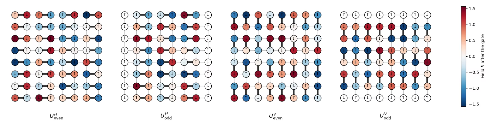
تشكّل الطبقات الفرعية الأربع دورة Floquet واحدة. تتكرر الدورة مرة مع الحقول نفسها، لذا تكون الديناميكيات عشوائية في المكان ودورية في الزمن. تبدأ الدائرة من حالة Néel، و هو نصف طول ضلع الشبكة. ترسم الخلية التالية دورة Floquet واحدة من شبكة العتاد ، طبقة فرعية بعد أخرى، مع حقول تشغيل العتاد، على نمط الشكل 5 من الورقة. الروابط السميكة هي بوابات كل طبقة فرعية. يُلوَّن كل كيوبت تعمل عليه بوابة بحسب الحقل العشوائي الذي يتلقاه بعدها، وتبقى الكيوبتات الخاملة بيضاء. تُظهر الأسهم حالة Néel الابتدائية، مع للحالة . يطبّق شكل الورقة الطبقات العمودية أولًا؛ ولا يُتوقع أن يغيّر أي من الترتيبين الفيزياء.
# circuit structure, 8x8 system:
side = 8
all_bonds = [bond for layer in brickwork_layers(side, side) for bond in layer]

# get the disorder parameters for a given system:
def sample_disorder(num_cols, num_rows, rng):
    # One pair of fields (h_i, h_j) per gate, reused in every Floquet cycle
    return [
        [
            (bond, tuple(rng.uniform(-np.pi / 2, np.pi / 2, 2)))
            for bond in layer
        ]
        for layer in brickwork_layers(num_cols, num_rows)
    ]

# build the structure for the 8x8 system
example_disorder = sample_disorder(
    side, side, np.random.default_rng(7)
)  # the hardware fields (section 4)
titles = [
    r"$U^H_\mathrm{even}$",
    r"$U^H_\mathrm{odd}$",
    r"$U^V_\mathrm{even}$",
    r"$U^V_\mathrm{odd}$",
]
norm = plt.Normalize(-np.pi / 2, np.pi / 2)
cmap = plt.get_cmap("RdBu_r")

fig, axes = plt.subplots(1, 4, figsize=(16, 4.8), layout="constrained")
for ax, title, sublayer in zip(axes, titles, example_disorder):
    for i, j in all_bonds:
        ax.plot(
            [i % side, j % side],
            [i // side, j // side],
            color="0.75",
            lw=1,
            zorder=0,
        )
    fields = {}
    for (i, j), (h_i, h_j) in sublayer:
        ax.plot(
            [i % side, j % side],
            [i // side, j // side],
            color="0.2",
            lw=4,
            zorder=1,
        )
        fields[i], fields[j] = h_i, h_j
    for q in range(side * side):
        x, y = q % side, q // side
        ax.scatter(
            x,
            y,
            s=260,
            color=cmap(norm(fields[q])) if q in fields else "white",
            edgecolor="black",
            zorder=2,
        )
        ax.text(
            x,
            y,
            "↓" if (x + y) % 2 else "↑",
            ha="center",
            va="center",
            fontsize=9,
            zorder=3,
        )
    ax.set_aspect("equal")
    ax.set_xlim(-1, side)  # padding, so the panels read as separate steps
    ax.set_ylim(side, -1)
    ax.axis("off")
    ax.set_title(title, y=-0.1, fontsize=13)
fig.colorbar(
    plt.cm.ScalarMappable(norm=norm, cmap=cmap),
    ax=axes,
    shrink=0.7,
    label="Field $h$ after the gate",
)
plt.show()
عرّف الحالة الابتدائية.
# initial state
def neel_state(circuit, num_cols, num_rows, layout):
    for y in range(num_rows):
        for x in range(num_cols):
            if (x + y) % 2 == 1:
                circuit.x(layout[y * num_cols + x])
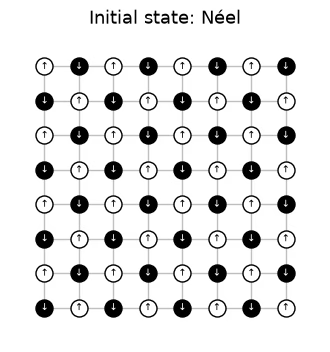
# The initial Néel state: |1⟩ (black, ↓) on odd sites, |0⟩ (white, ↑) on even sites

fig, ax = plt.subplots(figsize=(4, 4.4))
for i, j in all_bonds:
    ax.plot(
        [i % side, j % side],
        [i // side, j // side],
        color="0.75",
        lw=1,
        zorder=0,
    )
for q in range(side * side):
    x, y = q % side, q // side
    excited = (x + y) % 2 == 1
    ax.scatter(
        x,
        y,
        s=150,
        color="black" if excited else "white",
        edgecolor="black",
        zorder=2,
    )
    ax.text(
        x,
        y,
        "↓" if excited else "↑",
        ha="center",
        va="center",
        fontsize=7,
        color="white" if excited else "black",
        zorder=3,
    )
ax.set_aspect("equal")
ax.set_xlim(-1, side)
ax.set_ylim(side, -1)
ax.axis("off")
ax.set_title("Initial state: Néel", fontsize=13)
plt.show()
# actual circuit construction:
def heisenberg_floquet_circuit(
    num_cols, num_rows, coupling, num_cycles, disorder, measure=True
):
    num_qubits = num_cols * num_rows
    circuit = QuantumCircuit(num_qubits)
    neel_state(circuit, num_cols, num_rows, list(range(num_qubits)))
    cycle = QuantumCircuit(num_qubits)
    for sublayer in disorder:
        for (i, j), (h_i, h_j) in sublayer:
            heisenberg_gate(cycle, coupling, i, j, h_i, h_j)
    for _ in range(num_cycles):
        circuit.compose(cycle, inplace=True)
    if measure:
        circuit.measure_all()
    return circuit
مثال بحجم
تستخدم المحاكاة شبكة بدورتين، والاقترانات المدروسة في الورقة. تُعاد استخدام مجموعة واحدة من الحقول لكل اقتران.
# simulation parameters:
num_cols = num_rows = 4
num_qubits = num_cols * num_rows
num_cycles = 2
couplings = (
    np.array([0.005, 0.01, 0.02, 0.03, 0.04, 0.05, 0.06, 0.08, 0.10, 0.125])
    * np.pi
)
disorder = sample_disorder(num_cols, num_rows, np.random.default_rng(42))

# circuit construction:
logical_circuits = [
    heisenberg_floquet_circuit(
        num_cols, num_rows, coupling, num_cycles, disorder
    )
    for coupling in couplings
]
logical_circuits[5].draw(output="mpl", fold=-1)

# transpiling the circuit:
pass_manager = generate_preset_pass_manager(
    optimization_level=3,
    basis_gates=["cz", "rz", "sx", "x"],
    seed_transpiler=7,
)
circuits = [pass_manager.run(circuit) for circuit in logical_circuits]

def two_qubit_stats(circuit):
    count = sum(1 for inst in circuit.data if inst.operation.num_qubits == 2)
    depth = circuit.depth(lambda inst: inst.operation.num_qubits == 2)
    return count, depth

stats = {two_qubit_stats(circuit) for circuit in circuits}
assert len(stats) == 1, "the CZ structure should not depend on J"
num_cz, depth = stats.pop()
print(
    f"{num_qubits} qubits: {num_cz} CZ gates in {depth} layers, for every coupling"
)
circuits[5].draw("mpl", fold=-1, scale=0.4)
16 qubits: 144 CZ gates in 24 layers, for every coupling

لا حاجة إلى مُصرِّف ذكي، لأن الدوائر (والتجربة) صُمّمت لـ IBM Nighthawk.
حاكِ الشبكة
بالنسبة إلى الشبكة يمكنك فعل الأمرين: حساب الحالة الدقيقة عند كل اقتران، وأخذ عيّنات من كل دائرة بـ 10,000 لقطة، كما تفعل التجربة. تُخزَّن اللقطات بالشكل (دفعات، لقطات، كيوبتات)، وهو التخطيط نفسه للتوزيعات العشوائية في بيانات العتاد. هنا تشكّل اللقطات الـ 10,000 كلها دفعة واحدة، لذا لا يضيف bootstrap على الدفعات ضوضاء لقطات، ولا تُظهر أشرطة الخطأ في الرسم التالي سوى التباين بين مواضع الهوامش.
exact_states = [
    Statevector(
        heisenberg_floquet_circuit(
            num_cols, num_rows, c, num_cycles, disorder, measure=False
        )
    )
    for c in couplings
]

shots = 10_000
results = (
    StatevectorSampler(default_shots=shots, seed=1234).run(circuits).result()
)

# the output of the simulation for the 10 couplings
bits = [
    result.data.meas.to_bool_array(order="little").reshape(
        1, 10_000, num_qubits
    )
    for result in results
]

print(bits[0])
[[[False  True False ... False  True False]
  [False  True False ... False  True False]
  [False  True False ... False  True False]
  ...
  [False  True False ... False  True False]
  [False  True False ... False  True False]
  [False  True False ... False  True False]]]
2. ما الذي نقيسه وكيف نقدّره
IPR وإنتروبيا التصادم
لهامش من كيوبت مع توزيع سلاسل بتات ، الكمية المراد تقديرها هي نسبة المشاركة العكسية (IPR) للتوزيع الهامشي، ومنها إنتروبيا التصادم:
هي أيضًا احتمال أن تتفق لقطتان على الهامش. للحالة الجدائية ، وللحالة العشوائية ، لذا يتصاعد من 0 إلى نحو بت كلما صار الهامش عشوائيًا.
المقدِّر 1: عدّ أزواج اللقطات
Question. كيف تقدّر هذه الكمية من لقطاتك؟
الإجابة
يحسب المقدِّر الساذج كل من اللقطات بالصيغة ، ثم يجمع . هذا المقدِّر متحيّز.
يعدّ كل لقطة كأنها تتفق مع نفسها، مما يرفع التقدير: فهو يعطي في المتوسط بدلًا من . وبما أن هو احتمال أن تتفق لقطتان، فعُدّ فقط أزواج اللقطات المختلفة:
هذا غير متحيّز، وهو ما تحسبه ipr_from_shots أدناه.
# IPR expectation values:

# refactor this function cause it does not scale
def ipr_from_shots(bits):
    # Pair-counting estimate of the IPR of a marginal: the fraction of pairs of different shots
    # that agree on it. bits holds the marginal's qubits only, with shape (randomizations, shots,
    # qubits), and all randomizations are pooled.
    n = bits.shape[-1]
    outcomes = bits @ 2 ** np.arange(
        n
    )  # each shot's marginal bitstring, read as an integer
    counts = np.bincount(outcomes.ravel())  # how often each outcome occurs
    total = counts.sum()
    return float((counts * (counts - 1)).sum() / (total * (total - 1)))

def collision_entropy(ipr):
    return -np.log2(ipr)
المقدِّر 2: مفكوك بارسيفال
يمكن أيضًا كتابة IPR عبر التكافؤات لكل المجموعات الجزئية غير الفارغة من الهامش:
هذه الصيغة مهمة لأن طرق تخفيف الأخطاء مثل PEA تعمل على القيم المتوقعة، لا على الاحتمالات. كيوبت واحد: احتمالات النتائج هي و، لذا
هامش : إذا رمزنا لكيوبتاته بـ ، فإن للهامش تكافؤًا: 4 كيوبتات منفردة، و6 أزواج، و4 ثلاثيات، والهامش بأكمله، وبالتالي
def parity_supports(patch):
    # All nonempty subsets S of the marginal
    return sorted(
        [
            tuple(q for k, q in enumerate(patch) if mask & (1 << k))
            for mask in range(1, 1 << len(patch))
        ],
        key=len,
    )

def parity_expectation_values(bits, supports):
    # Shot-averaged <Z_S> for every support, per randomization
    signs = 1 - 2 * bits.astype(np.int8)
    return np.stack(
        [signs[..., list(s)].prod(axis=-1).mean(axis=-1) for s in supports],
        axis=-1,
    )

# Example: the parities of a 3-qubit marginal made of lattice qubits 5, 6, and 9
print(parity_supports([5, 6, 9]))
print(f"A 3×3 marginal has {len(parity_supports(range(9)))} parities")
[(5,), (6,), (9,), (5, 6), (5, 9), (6, 9), (5, 6, 9)]
A 3×3 marginal has 511 parities
المتوسط على الهوامش
دوال مفيدة إضافية: قيم Haar، واختيار الهوامش، وإعادة العينات (bootstrapping)، وحساب المتوسطات.
# functions for the Haar values on plots:
def haar_ipr(num_patch, num_qubits):
    # Mean IPR of a marginal for Haar-random states in the sector with num_qubits // 2 ones
    weight = num_qubits // 2
    dimension = comb(num_qubits, weight)
    total = 0
    for k in range(num_patch + 1):  # k ones on the marginal
        rest = (
            comb(num_qubits - num_patch, weight - k) if weight - k >= 0 else 0
        )
        total += comb(num_patch, k) * rest * (rest + 1)
    return total / (dimension * (dimension + 1))

def haar_entropy(num_patch, num_qubits):
    return collision_entropy(haar_ipr(num_patch, num_qubits))

# definitions of positions in the lattice:
def patch_qubits(anchor, shape, num_cols):
    # Lattice indices of a rectangular marginal with its top-left corner at anchor
    (x0, y0), (width, height) = anchor, shape
    return [
        (y0 + dy) * num_cols + (x0 + dx)
        for dy in range(height)
        for dx in range(width)
    ]

def all_positions(shape, num_cols, num_rows):
    # Every placement of a (width, height) marginal on the lattice
    width, height = shape
    return [
        patch_qubits((x, y), shape, num_cols)
        for y in range(num_rows - height + 1)
        for x in range(num_cols - width + 1)
    ]

# bootstrapping for error bars:
bootstrap_rng = np.random.default_rng(0)

def bootstrap_error(statistic, *samples, axis=0, num_resamples=50):
    # Shot noise of a statistic, from resampling the randomizations (along axis of every
    # sample) with replacement
    values = []
    for _ in range(num_resamples):
        resampled = [
            np.take(
                x,
                bootstrap_rng.integers(0, x.shape[axis], x.shape[axis]),
                axis=axis,
            )
            for x in samples
        ]
        values.append(statistic(*resampled))
    return float(np.std(values, ddof=1))

# averaging the ipr over marginals:
def average_ipr(iprs, shot_errors):
    # iprs and shot_errors have shape (positions, couplings). The mean IPR over positions, and its
    # error: the spread between positions plus the shot noise of each (law of total variance)
    iprs, shot_errors = np.asarray(iprs), np.asarray(shot_errors)
    count = len(iprs)
    variance = (
        iprs.var(axis=0, ddof=1) / count
        + (shot_errors**2).sum(axis=0) / count**2
    )
    return iprs.mean(axis=0), np.sqrt(variance)
# Calculating exact simulation entropies:
patch_shapes = {
    "1×1": (1, 1),
    "1×2": (2, 1),
    "2×2": (2, 2),
    "2×3": (3, 2),
    "3×3": (3, 3),
}

# calculate the exact entropies:
sim_positions = {
    label: all_positions(shape, num_cols, num_rows)
    for label, shape in patch_shapes.items()
}
exact_iprs = {  # shape (positions, couplings)
    label: np.array(
        [
            [(s.probabilities(qargs=q) ** 2).sum() for s in exact_states]
            for q in qubit_lists
        ]
    )
    for label, qubit_lists in sim_positions.items()
}
exact_entropies = {
    label: collision_entropy(v.mean(axis=0))
    for label, v in exact_iprs.items()
}

# Average IPR of every shape over its positions, from the sampled shots, then the entropy
iprs_from_shots = {}  # per shape: average IPR and its error, at every coupling
entropies_from_shots = {}  # per shape: average entropy and its error, at every coupling
for label, qubit_lists in sim_positions.items():
    iprs = [[ipr_from_shots(b[:, :, q]) for b in bits] for q in qubit_lists]

    # bootstrapping over subsampling for error bars:
    errors = [
        [bootstrap_error(ipr_from_shots, b[:, :, q]) for b in bits]
        for q in qubit_lists
    ]
    ipr, ipr_error = average_ipr(iprs, errors)
    iprs_from_shots[label] = (ipr, ipr_error)
    entropies_from_shots[label] = (
        collision_entropy(ipr),
        ipr_error / (ipr * np.log(2)),
    )
# Now plot the average IPR on the left, and the same averages as entropies on the right
colors = plt.cm.plasma(np.linspace(0.05, 0.8, len(patch_shapes)))
fig, (ax_ipr, ax_entropy) = plt.subplots(1, 2, figsize=(12.8, 4.2))
for (label, qubit_lists), color in zip(sim_positions.items(), colors):
    n = len(qubit_lists[0])
    ipr, ipr_error = iprs_from_shots[label]
    entropy, entropy_error = entropies_from_shots[label]
    # Left: the average IPR, with its exact value and its random-state value
    ax_ipr.axhline(haar_ipr(n, num_qubits), color=color, ls="dashdot", lw=0.9)
    ax_ipr.plot(
        couplings / np.pi, exact_iprs[label].mean(axis=0), color=color
    )
    ax_ipr.errorbar(
        couplings / np.pi,
        ipr,
        yerr=ipr_error,
        fmt="o",
        color=color,
        mec="white",
        ms=7,
        capsize=3,
        label=f"{label} ({len(qubit_lists)} positions)",
    )
    # Right: the average collision entropy
    ax_entropy.axhline(
        haar_entropy(n, num_qubits), color=color, ls="dashdot", lw=0.9
    )
    ax_entropy.plot(couplings / np.pi, exact_entropies[label], color=color)
    ax_entropy.errorbar(
        couplings / np.pi,
        entropy,
        yerr=entropy_error,
        fmt="o",
        color=color,
        mec="white",
        ms=7,
        capsize=3,
        label=f"{label} ({len(qubit_lists)} positions)",
    )
ax_ipr.set_yscale("log")
ax_ipr.set_ylabel("Average IPR")
ax_entropy.set_ylabel("Average collision entropy (bits)")
for ax in (ax_ipr, ax_entropy):
    ax.set_xlabel("Coupling $J/\\pi$")
fig.suptitle("Exact (lines) and sampled (dots), 4×4 lattice, 2 cycles")
ax_entropy.legend(title="Marginal", loc="upper left")
fig.tight_layout()
plt.show()
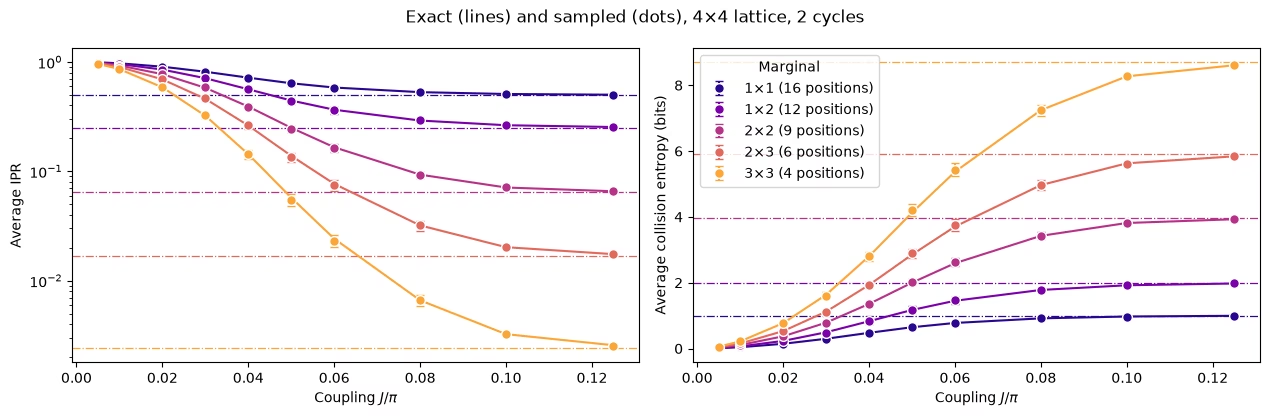
يرتفع كل شكل من أشكال الهوامش بسلاسة نحو قيمته للحالة العشوائية، وتصل الهوامش الأكبر إلى ذلك عند قيم أكبر.
3. الضوضاء وكيف نتخلص منها
محاكاة مع ضوضاء
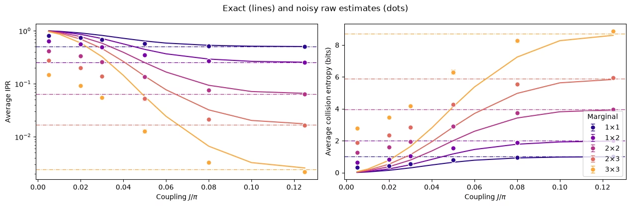
الآن أضف الضوضاء: ضوضاء إزالة استقطاب بنسبة 1% على كل بوابتين CZ، وخطأ قراءة بنسبة 3% على كل كيوبت، مع أخذ العينات بواسطة Sampler من Qiskit Aer. مع وجود 144 بوابة CZ في الدائرة، تكون هذه الضوضاء أقل بكثير مما تراه دوائر العتاد 8×8، لكنها كافية لنرى تأثيرها. تستخدم المحاكاة ستة اقترانات و4,000 لقطة (shot) لكل منها، وتستغرق نحو 1.5 دقيقة.
سؤال. قبل أن تشغّلها: هل ستجعل الضوضاء النظام يبدو أكثر ترمّلًا حراريًا (thermalized) أم أقل؟
الإجابة
أكثر. تشوّش الضوضاء النتائج، فتدفع كل توزيع هامشي نحو التوزيع المنتظم، فينخفض IPR الخام وترتفع الإنتروبيا. وبدون تخفيف، تبدو الضوضاء كأنها حرارة توازن (thermalization) غير موجودة فعلًا، وتظهر نقاط التقاطع مبكرة جدًا.
# define the noise model

noise_model = NoiseModel()
# two qubit depolarizing noise:
noise_model.add_all_qubit_quantum_error(depolarizing_error(0.01, 2), ["cz"])
# symmetric readout noise:
noise_model.add_all_qubit_readout_error(
    ReadoutError([[0.97, 0.03], [0.03, 0.97]])
)

# simulation is done using trajectories
noisy_sampler = AerSampler(
    default_shots=4000,
    seed=1,
    options={"backend_options": {"noise_model": noise_model}},
)

# choose a subset of J values for speed:
noisy_indices = [
    0,
    2,
    3,
    5,
    7,
    9,
]  # J/π = 0.005, 0.02, 0.03, 0.05, 0.08, 0.125
noisy_results = noisy_sampler.run(
    [circuits[k] for k in noisy_indices]
).result()

# No twirling here, so the 20 "randomizations" are just batches of 200 shots
noisy_bits = {
    k: result.data.meas.to_bool_array(order="little").reshape(
        20, 200, num_qubits
    )
    for k, result in zip(noisy_indices, noisy_results)
}
# Calculating noisy entropies

# Average IPR of every shape over its positions, from the noisy shots, then the entropy
noisy_iprs = {}  # per shape: average IPR and its error, at every noisy coupling
noisy_entropies = {}  # per shape: average entropy and its error, at every noisy coupling
for label, qubit_lists in sim_positions.items():
    iprs = [
        [ipr_from_shots(noisy_bits[k][:, :, q]) for k in noisy_indices]
        for q in qubit_lists
    ]

    # bootstrapping over subsampling for error bars:
    errors = [
        [
            bootstrap_error(ipr_from_shots, noisy_bits[k][:, :, q])
            for k in noisy_indices
        ]
        for q in qubit_lists
    ]
    ipr, ipr_error = average_ipr(iprs, errors)
    noisy_iprs[label] = (ipr, ipr_error)
    noisy_entropies[label] = (
        collision_entropy(ipr),
        ipr_error / (ipr * np.log(2)),
    )
fig, (ax_ipr, ax_entropy) = plt.subplots(1, 2, figsize=(12.8, 4.2))
for (label, qubit_lists), color in zip(sim_positions.items(), colors):
    n = len(qubit_lists[0])
    ipr, ipr_error = noisy_iprs[label]
    entropy, entropy_error = noisy_entropies[label]
    # Left: the average IPR, with its exact value and its random-state value
    ax_ipr.axhline(haar_ipr(n, num_qubits), color=color, ls="dashdot", lw=0.9)
    ax_ipr.plot(
        couplings / np.pi, exact_iprs[label].mean(axis=0), color=color
    )
    ax_ipr.errorbar(
        couplings[noisy_indices] / np.pi,
        ipr,
        yerr=ipr_error,
        fmt="o",
        color=color,
        mec="white",
        ms=7,
        capsize=3,
        label=label,
    )
    # Right: the same averages as entropies
    ax_entropy.axhline(
        haar_entropy(n, num_qubits), color=color, ls="dashdot", lw=0.9
    )
    ax_entropy.plot(couplings / np.pi, exact_entropies[label], color=color)
    ax_entropy.errorbar(
        couplings[noisy_indices] / np.pi,
        entropy,
        yerr=entropy_error,
        fmt="o",
        color=color,
        mec="white",
        ms=7,
        capsize=3,
        label=label,
    )
ax_ipr.set_yscale("log")
ax_ipr.set_ylabel("Average IPR")
ax_entropy.set_ylabel("Average collision entropy (bits)")
for ax in (ax_ipr, ax_entropy):
    ax.set_xlabel("Coupling $J/\\pi$")
fig.suptitle("Exact (lines) and noisy raw estimates (dots)")
ax_entropy.legend(title="Marginal", loc="lower right")
fig.tight_layout()
plt.show()
عصف ذهني: كيف ستتخلص من هذا؟
النهج المقترح
عند صغيرة، تكون الحالة متشابكة بالكاد، فيكون الجواب المثالي هناك رخيصًا حسابيًا بالطرق الكلاسيكية، حتى مع 64 كيوبت. وهذا يوحي بقياس أثر الضوضاء عند اقتران معايرة صغير وتصحيح كل اقتران آخر به. هناك طريقتان طبيعيتان لذلك، تُسميان المعايرة منخفضة التشابك (LEC):
LEC على IPR. أعد تحجيم زيادة IPR عن قيمته للتوزيع المنتظم، ، بعامل واحد لكل هامش:
LEC على القيم المتوقعة . أعد تحجيم كل تكافؤ من الهامش بعامله الخاص، ثم أعد بناء IPR بصيغة Parseval:
في الشيفرة، يُزال انحياز كل تكافؤ مُعاد تحجيمه ومربّع بطرح تباينه، كما في القسم 2.
الطريقتان متطابقتان إذا كان كل يساوي .
Question. What are the pros and cons of these methods?
الإجابة
Pros
-
رخيصة: لا حاجة لبيانات إضافية من الجهاز، فقط محاكاة كلاسيكية عند .
-
تستفيد من بنية الدائرة: عمق الدائرة وطبقات CZ لا تتغير مع ، لذا فإن الضوضاء عند هي نفسها عند كل آخر.
Cons
- تفترض أن أثر الضوضاء على القيم المرصودة لا يعتمد على : الضوضاء نفسها ثابتة، لكن كيفية إخمادها لـ IPR أو لكل قد تتغير مع نمو .
الطريقتان على المحاكاة ذات الضوضاء
# function to mitigate the IPR signal:
def mitigate_ipr_w_lec(
    ipr_raw, ipr_raw_calibration, ipr_ideal_calibration, num_patch
):
    # LEC on the IPR: one factor R0 for the excess over the uniform value
    uniform = 2.0**-num_patch
    factor = (ipr_ideal_calibration - uniform) / (
        ipr_raw_calibration - uniform
    )
    return uniform + factor * (ipr_raw - uniform)

# function used to calculate the target <Z> expectation values
def parities_from_probabilities(probabilities):
    # Ideal <Z_S> from a marginal distribution, in parity_supports order: subsets
    # by size, and in bitmask order within each size
    outcomes = np.arange(len(probabilities))
    masks = np.array(sorted(range(1, len(probabilities)), key=int.bit_count))
    signs = (-1.0) ** np.bitwise_count(outcomes[:, None] & masks[None, :])
    return np.asarray(probabilities) @ signs

# calculate boosting factors:
def lec_z_factors(calibration_parities, ideal_parities):
    # LEC on <Z>: one factor r_S per parity, from data with shape (randomizations, supports).
    return ideal_parities / calibration_parities.mean(axis=0)

# function to mitigate the IPR from <Z> expectation values:
def mitigate_ipr_w_lec_on_parities(
    parities, calibration_parities, ideal_calibration_parities, num_patch
):
    # LEC on <Z>: rescale each parity by its factor r_S = ideal / raw at J0, then rebuild the IPR
    # with Parseval. parities and calibration_parities have shape (randomizations, supports).
    # Each squared, rescaled parity is debiased by subtracting its variance, which to first
    # order combines the shot noise at J. The shot noise of r_S from J0 is omitted; including it
    # does not change the results.
    factors = lec_z_factors(calibration_parities, ideal_calibration_parities)
    mean = parities.mean(axis=0)  # mean over the twirling instances
    variance = parities.var(axis=0, ddof=1) / len(
        parities
    )  # variance of the mean
    rescaled = factors * mean
    rescaled_variance = factors**2 * variance
    return float((1 + np.sum(rescaled**2 - rescaled_variance)) / 2**num_patch)
def lec_estimates(patch_bits, parities, ideal, calibration, num_patch):
    # LEC on the IPR and on <Z> for one marginal position, at every coupling: values and shot
    # noise. patch_bits (the bits of the marginal only) and parities are per coupling, with
    # randomizations first.
    q_ideal = (ideal**2).sum()
    ideal_parities = parities_from_probabilities(ideal)

    def ipr_statistic(b, c):
        return mitigate_ipr_w_lec(
            ipr_from_shots(b), ipr_from_shots(c), q_ideal, num_patch
        )

    def z_statistic(p, c):
        return mitigate_ipr_w_lec_on_parities(p, c, ideal_parities, num_patch)

    values = {"LEC on IPR": [], "LEC on ⟨Z⟩": []}
    errors = {"LEC on IPR": [], "LEC on ⟨Z⟩": []}
    for k in range(len(patch_bits)):
        if (
            k == calibration
        ):  # both match the ideal value at J0 by construction
            for method in values:
                values[method].append(q_ideal)
                errors[method].append(0.0)
            continue
        values["LEC on IPR"].append(
            ipr_statistic(patch_bits[k], patch_bits[calibration])
        )
        errors["LEC on IPR"].append(
            bootstrap_error(
                ipr_statistic, patch_bits[k], patch_bits[calibration]
            )
        )
        values["LEC on ⟨Z⟩"].append(
            z_statistic(parities[k], parities[calibration])
        )
        errors["LEC on ⟨Z⟩"].append(
            bootstrap_error(z_statistic, parities[k], parities[calibration])
        )
    return values, errors

# getting all the data:
calibration_index = 0  # index of J0 = 0.005π in noisy_indices
mitigated = {
    "LEC on IPR": {},
    "LEC on ⟨Z⟩": {},
}  # per shape: (values, errors), each (positions, couplings)
for label, qubit_lists in sim_positions.items():
    n = len(qubit_lists[0])
    per_position = []
    for qubits in qubit_lists:
        supports = parity_supports(qubits)
        parities = [
            parity_expectation_values(noisy_bits[k], supports)
            for k in noisy_indices
        ]
        patch_bits = [noisy_bits[k][:, :, qubits] for k in noisy_indices]
        ideal = exact_states[noisy_indices[calibration_index]].probabilities(
            qargs=qubits
        )
        per_position.append(
            lec_estimates(patch_bits, parities, ideal, calibration_index, n)
        )
    for method in mitigated:
        mitigated[method][label] = (
            [p[0][method] for p in per_position],
            [p[1][method] for p in per_position],
        )

# Average over positions, then the entropy, for both methods
mitigated_entropies = {
    method: {} for method in mitigated
}  # per method and shape: entropy and its error
for method, by_shape in mitigated.items():
    for label, (values, errors) in by_shape.items():
        ipr, ipr_error = average_ipr(values, errors)
        mitigated_entropies[method][label] = (
            collision_entropy(ipr),
            ipr_error / (ipr * np.log(2)),
        )  # log here comes from error propagation
# Plot the data mitigated with both methods:

fig, axes = plt.subplots(1, 2, figsize=(12.8, 4.2), sharey=True)
for ax, (method, by_shape) in zip(axes, mitigated_entropies.items()):
    for (label, qubit_lists), color in zip(sim_positions.items(), colors):
        entropy, error = by_shape[label]
        ax.axhline(
            haar_entropy(len(qubit_lists[0]), num_qubits),
            color=color,
            ls="dashdot",
            lw=0.9,
        )
        ax.plot(couplings / np.pi, exact_entropies[label], color=color)
        ax.errorbar(
            couplings[noisy_indices] / np.pi,
            entropy,
            yerr=error,
            fmt="o",
            color=color,
            mec="white",
            ms=7,
            capsize=3,
            label=label,
        )
    ax.set_title(f"{method} (lines: exact)")
    ax.set_xlabel("Coupling $J/\\pi$")
axes[0].set_ylabel("Average collision entropy (bits)")
axes[0].legend(title="Marginal", loc="lower right")
fig.tight_layout()
plt.show()

# add the noisy data here too
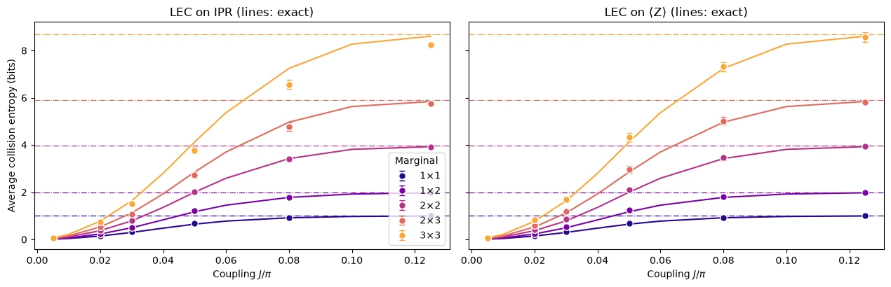
تزيل الطريقتان معظم الضرر: التقديرات الخام في الرسم السابق عشوائية جدًا، أما المخففة فتتبع المنحنيات الدقيقة. وتظهر الفروق في الهوامش الكبيرة.
مع الهوامش الصغيرة تعمل الطريقتان. أما مع الهامش فإن LEC على أقرب بوضوح.
لماذا تعطي LEC على IPR إنتروبيا أقل مما يجب. الإنتروبيا الأقل تعني أن IPR أكبر مما يجب: LEC على IPR تضخّمه أكثر من اللازم. فهي تفترض أن الضوضاء تخمد مساهمة كل في IPR بالعامل نفسه. عند تكون كل قريبة من ، فتساهم كل السلاسل بالتساوي، ومعظم السلاسل ذات وزن متوسط: من بين 511 سلسلة في هامش هناك 252 ذات وزن 4 أو 5، وتسع فقط ذات وزن 1. تخمد الضوضاء السلسلة أكثر كلما ارتفع وزنها (خطأ القراءة وحده يخمد سلسلة وزنها بالعامل )، لذا فإن العامل الوحيد يتحدد أساسًا بإخماد السلاسل متوسطة الوزن. ومع نمو تضمحل ذات الوزن الأعلى أسرع، ويصبح IPR محمولًا أكثر فأكثر على سلاسل منخفضة الوزن، وتخمدها الضوضاء أقل. وتعزيزها بعامل تعلّمناه أساسًا من سلاسل مُخمَدة بقوة أكبر يضخّم IPR أكثر من اللازم. ويزداد الأثر مع حجم الهامش، لأن الهامش الأكبر له مدى أوسع من الأوزان. ويبلغ أقصاه عند المتوسطة، بعد أن يتغير مزيج السلاسل لكن بينما لا تزال زيادة IPR عن قيمته المنتظمة مهمة.
لماذا تخطئ LEC على في الاتجاه المعاكس. إنها تعيد تحجيم كل سلسلة بعاملها الخاص، فلا يؤثر فيها الانتقال بين الأوزان. هي تفترض فقط أن كل سلسلة تحتفظ بإخمادها عند . ومع نمو ينتشر كل إلى مؤثرات ذات وزن أعلى، تلتقط ضوضاء أكثر مما عند ، فتصحّح العوامل أقل قليلًا من اللازم وتأتي الإنتروبيا أعلى قليلًا مما يجب.
إذن التنبؤ الذي نختبره على العتاد هو: كلما كبر الهامش، زادت أفضلية LEC على . على العتاد تكون الضوضاء أقوى وليست من شكل معروف.
4. التشغيل على نطاق واسع
تُشغّل تجربة العتاد شبكة بأربع دورات: 64 كيوبت و1,344 بوابة CZ في 48 طبقة، عند تسعة اقترانات. تتغير خمسة أشياء مقارنة بالمحاكاة:
-
يجب تعلّم الضوضاء، وهذا لا ينجح إلا إذا كانت طبقات CZ ثابتة.
-
التدوير العشوائي (Twirling) يحوّل ضوضاء كل طبقة إلى قناة Pauli، يمكن تعلّمها وتضخيمها.
-
الفصل الديناميكي (DD) يحمي الكيوبتات الخاملة.
-
تضخيم الضوضاء لـ PEA يُنفَّذ في المهمة نفسها مع البيانات الرئيسية.
-
محاكاة MPS عند صغيرة توفّر المراجع الكلاسيكية لتخفيف الأخطاء المعتمد على LEC.
الخلايا التي تحتاج إلى backend لا تعمل إلا عندما تكون RUN_ON_HARDWARE مساوية لـ True. ويمكن إعادة تشغيل محاكاة MPS بضبط COMPUTE_MPS_REFERENCES على True. أما بقية الخلايا فتعمل هنا.
# hardware run parameters:
num_cols_hw = num_rows_hw = 8
num_qubits_hw = num_cols_hw * num_rows_hw
num_cycles_hw = 4
couplings_hw = (
    np.array([0.005, 0.01, 0.02, 0.03, 0.05, 0.07, 0.09, 0.11, 0.125]) * np.pi
)
calibration_hw = 0  # J0 = 0.005π
disorder_hw = sample_disorder(
    num_cols_hw, num_rows_hw, np.random.default_rng(7)
)

# if running PEA:
noise_factors = np.array([1.0, 1.5, 2.0])  # PEA noise-amplification factors
طبقات CZ الثابتة
def compile_by_sublayer(
    num_cols,
    num_rows,
    coupling,
    num_cycles,
    disorder,
    pass_manager,
    layout=None,
    num_physical_qubits=None,
):
    # Compile each sublayer once and repeat it with barriers, so the CZ layers are the
    # same in every cycle and at every coupling. The registers are named explicitly
    # because register names enter Samplomatic's box hashes. Bits land in lattice order.
    num_qubits = num_cols * num_rows
    if layout is None:
        layout, num_physical_qubits = list(range(num_qubits)), num_qubits
    blocks = []
    for sublayer in disorder:
        block = QuantumCircuit(num_qubits)
        for (i, j), (h_i, h_j) in sublayer:
            heisenberg_gate(block, coupling, i, j, h_i, h_j)
        blocks.append(pass_manager.run(block))
    circuit = QuantumCircuit(
        QuantumRegister(num_physical_qubits, "q"),
        ClassicalRegister(num_qubits, "meas"),
    )
    neel_state(circuit, num_cols, num_rows, layout)
    for _ in range(num_cycles):
        for block in blocks:
            circuit.compose(block, inplace=True)
            circuit.barrier(layout)
    circuit.measure(layout, range(num_qubits))
    return circuit
صناديق لتعلّم الضوضاء
ثم يجمّع مدير تمريرات التصنيد (boxing) في Samplomatic كل دائرة في صناديق: صندوق لكل طبقة CZ وصندوق للقياسات. يحمل كل صندوق إشارة إلى نموذج الضوضاء الذي يحتاجه، فيمكنك التحقق من أن كل الاقترانات تتشارك الصناديق نفسها. تنفّذ الخلية التالية ذلك لدوائر الخاصة بتشغيل العتاد، بعد تجميعها إلى بوابات CZ دون backend، وتطبع الصناديق التي سيوصّفها تعلّم الضوضاء.
from samplomatic import build
from samplomatic.transpiler import generate_boxing_pass_manager
from samplomatic.utils import find_unique_box_instructions

boxing_pass_manager = generate_boxing_pass_manager(
    enable_gates=True,  # twirl the CZ layers
    enable_measures=True,  # twirl the measurements
    inject_noise_targets="gates",  # PEA amplifies the noise of the CZ layers only
    inject_noise_strategy="uniform_modification",
)

def noise_refs(boxed_circuit):
    return sorted(
        annotation.ref
        for box in find_unique_box_instructions(boxed_circuit.data)
        for annotation in box.operation.annotations
        if hasattr(annotation, "ref")
    )

# The 8x8 hardware circuits, compiled to CZ gates on the lattice qubits (no backend needed)
compiled_8x8 = [
    compile_by_sublayer(
        num_cols_hw, num_rows_hw, c, num_cycles_hw, disorder_hw, pass_manager
    )
    for c in couplings_hw
]
boxed_8x8 = [boxing_pass_manager.run(circuit) for circuit in compiled_8x8]
assert all(
    noise_refs(b) == noise_refs(boxed_8x8[0]) for b in boxed_8x8
), "layers differ between couplings"
num_cz, depth = two_qubit_stats(compiled_8x8[0])
print(
    f"{num_qubits_hw} qubits: {num_cz} CZ gates in {depth} layers, for every coupling"
)
for box in find_unique_box_instructions(boxed_8x8[0].data):
    ops = box.operation.blocks[0].count_ops()
    print(
        f"{box.operation.num_qubits}-qubit box: {ops.get('cz', 0)} CZ, {ops.get('measure', 0)} measurements"
    )
print(
    f"All {len(boxed_8x8)} couplings share these {len(find_unique_box_instructions(boxed_8x8[0].data))} boxes"
)
64 qubits: 1344 CZ gates in 48 layers, for every coupling
64-qubit box: 32 CZ, 0 measurements
64-qubit box: 24 CZ, 0 measurements
64-qubit box: 32 CZ, 0 measurements
64-qubit box: 24 CZ, 0 measurements
64-qubit box: 0 CZ, 64 measurements
All 9 couplings share these 5 boxes
تدوير الدوائر عشوائيًا (Twirl)
في كل عملية عشوائية، يضع Samplomatic بوابات Pauli عشوائية قبل كل صندوق وبوابات التعويض بعده، مدمجة في بوابات الكيوبت الواحد المجاورة. وعند أخذ المتوسط على العشوائيات تصبح ضوضاء كل طبقة قناة Pauli، يمكن لـ NoiseLearnerV3 تعلّمها كنموذج Pauli-Lindblad متناثر، ويمكن لخطوة PEA تضخيمها. أما تدوير القياس العشوائي فيقلب البتات عشوائيًا قبل القراءة. وتُلغى هذه القلبات برمجيًا، مما يجعل ضوضاء القراءة متناظرة وهو أساس تصحيح القراءة (TREX).
سير عمل العتاد
اختر الكيوبتات، وجمّع الدوائر، ثم تعلّم الضوضاء وشغّل المسح. هذه الخلايا معطّلة هنا.
اختر الكيوبتات. تتسع الشبكة المربعة في Nighthawk لشبكة دون بوابات SWAP. تقيّم الخلية كل مستطيل في الشبكة بحسب أخطاء CZ والقراءة المبلّغ عنها وتختار الأفضل.
def square_layouts(backend, side):
    # Every side x side rectangle of the square qubit grid that supports all bonds
    target = backend.target

    def has_cz(a, b):
        return (a, b) in target["cz"] or (b, a) in target["cz"]

    stride = next(
        s
        for s in (10, 12)
        if all(has_cz(q, q + s) for q in range(backend.num_qubits - s))
    )
    layouts = []
    for y0 in range(backend.num_qubits // stride - side + 1):
        for x0 in range(stride - side + 1):
            layout = [
                stride * (y0 + y) + x0 + x
                for y in range(side)
                for x in range(side)
            ]
            bonds = [
                bond
                for layer in brickwork_layers(side, side)
                for bond in layer
            ]
            if all(has_cz(layout[i], layout[j]) for i, j in bonds):
                layouts.append(((x0, y0), layout))
    return layouts

def layout_score(backend, layout, side, uses_per_bond):
    # Minus the summed log-fidelity of the bonds (each used uses_per_bond times) and readouts
    properties, target = backend.properties(), backend.target
    cz_errors = []
    for i, j in (
        bond for layer in brickwork_layers(side, side) for bond in layer
    ):
        pair = (
            (layout[i], layout[j])
            if (layout[i], layout[j]) in target["cz"]
            else (layout[j], layout[i])
        )
        cz_errors.append(properties.gate_error("cz", pair))
    readout_errors = [properties.readout_error(q) for q in layout]
    if max(cz_errors) >= 0.5 or max(readout_errors) >= 0.25:
        return np.inf  # an unusable qubit or bond
    return float(
        -uses_per_bond * np.log1p(-np.array(cz_errors)).sum()
        - np.log1p(-np.array(readout_errors)).sum()
    )

if RUN_ON_HARDWARE:
    from qiskit_ibm_runtime import QiskitRuntimeService

    def holds_lattice(backend):
        try:
            return bool(square_layouts(backend, num_cols_hw))
        except (KeyError, StopIteration):
            return False

    service = QiskitRuntimeService()
    candidates = [
        b
        for b in service.backends(operational=True, simulator=False)
        if holds_lattice(b)
    ]
    backend = min(candidates, key=lambda b: b.status().pending_jobs)
    score, origin, initial_layout = min(
        (
            layout_score(backend, layout, num_cols_hw, 3 * num_cycles_hw),
            origin,
            layout,
        )
        for origin, layout in square_layouts(backend, num_cols_hw)
    )
    print(f"{backend.name}: origin {origin}, score {score:.2f}")
التجميع. الخطوات نفسها كما سبق على الكيوبتات المختارة، يليها build، الذي يحوّل كل دائرة مصنّدة إلى دائرة قالب وsamplex، وهو الوصفة لسحب بوابات التدوير والضوضاء المحقونة. ويُضاف DD إلى القوالب.
if RUN_ON_HARDWARE:
    from qiskit_ibm_runtime.executor.dynamical_decoupling import (
        generate_dd_pass_manager,
    )
    from qiskit_ibm_runtime.options import DynamicalDecouplingOptions

    # PEA structure functions:
    target_pass_manager = generate_preset_pass_manager(
        target=backend.target,
        optimization_level=3,
        initial_layout=initial_layout,
        routing_method="none",
        seed_transpiler=7,
    )
    boxed_hw = [
        boxing_pass_manager.run(
            compile_by_sublayer(
                num_cols_hw,
                num_rows_hw,
                coupling,
                num_cycles_hw,
                disorder_hw,
                target_pass_manager,
                layout=initial_layout,
                num_physical_qubits=backend.num_qubits,
            )
        )
        for coupling in couplings_hw
    ]
    assert all(noise_refs(b) == noise_refs(boxed_hw[0]) for b in boxed_hw)
    unique_boxes_hw = find_unique_box_instructions(boxed_hw[0].data)

    # DD pass:
    dd_pass_manager = generate_dd_pass_manager(
        backend,
        DynamicalDecouplingOptions(
            enable=True,
            sequence_type="XY4",
            scheduling_method="alap",
            extra_slack_distribution="middle",
            skip_reset_qubits=False,
        ),
    )
    templates = []
    for circuit in boxed_hw:
        template, samplex = build(circuit)
        templates.append((dd_pass_manager.run(template), samplex))
تعلّم الضوضاء وتشغيل المسح. تتعلم مهمة NoiseLearnerV3 واحدة الصناديق الخمسة كلها: نموذج Pauli-Lindblad لكل طبقة من طبقات CZ الأربع، وضوضاء القراءة لصندوق القياس. ثم يحتوي QuantumProgram واحد على الاقترانات التسعة كلها. يحصل كل عنصر على قالبه وsamplex الخاص به ونماذج الضوضاء المتعلَّمة وثلاثة مقاييس للضوضاء. المقياس 0 هو البيانات غير المضخّمة لطريقتي LEC. أما المقياسان 0.5 و1 فيضيفان 50% و100% من الضوضاء المتعلَّمة لـ PEA، التي تستقرئ للعودة إلى انعدام الضوضاء. يستخدم هذا نحو 40 ثانية من وقت QPU.
if RUN_ON_HARDWARE:
    from qiskit_ibm_runtime import Executor, NoiseLearnerV3, QuantumProgram

    # Learn the noise of the five boxes
    learner = NoiseLearnerV3(backend)
    learner.options.num_randomizations = 32
    learner.options.shots_per_randomization = 128
    # Up to 24 layer pairs, the depth of the 48-layer circuits
    learner.options.layer_pair_depths = [0, 1, 2, 4, 16, 24]
    learner_job = learner.run(unique_boxes_hw)
    print("Noise learning job:", learner_job.job_id())

    # Run the sweep, with the learned noise amplified by each of the noise factors
    noise_maps = learner_job.result().to_dict(
        instructions=unique_boxes_hw, require_refs=False
    )
    program = QuantumProgram(shots=200)
    for template, samplex in templates:
        program.append_samplex_item(
            template,
            samplex=samplex,
            samplex_arguments={
                "pauli_lindblad_maps": noise_maps,
                **{
                    f"noise_scales.{ref}": (noise_factors - 1).reshape(-1, 1)
                    for ref in noise_maps
                },
            },
            shape=(len(noise_factors), 200),  # noise scales x randomizations
        )
    executor_job = Executor(backend).run(program)
    print("Executor job:", executor_job.job_id())
    # Section 5 converts the results of these two jobs and saves them
5. بيانات العتاد
يستكشف هذا القسم أداء الطرق السابقة على بيانات عتاد حقيقية من معالج Nighthawk.
تحميل التشغيل
عندما تكون RUN_ON_HARDWARE مساوية لـ True، تحوّل الخلية التالية نتائج المهمتين من القسم 4 وتحفظها في data/hardware_run_new.npz بالصيغة نفسها للتشغيل المحفوظ، ليمكن تحليل التشغيل الجديد لاحقًا. وإلا فإنها تحمّل التشغيل المحفوظ من data/hardware_run.npz. تُحزَم البتات على طول محور الكيوبت لتوفير المساحة.
إذا أُعيد تشغيل النواة (kernel) أثناء عمل المهام، فلا تُرسلها من جديد. أعد تشغيل الخلايا التي تسبق آخر استدعاء في القسم 4، وتحقق من اختيار الكيوبتات نفسها، واضبط learner_job وexecutor_job على service.job(job_id) بمعرّفات المهام التي طُبعت في القسم 4.
if RUN_ON_HARDWARE:

    def unflip(item_result):
        # Undo the measurement twirling of an Executor item: flip back the bits that were flipped
        return item_result["meas"] ^ item_result["measurement_flips.meas"]

    learner_result = learner_job.result()
    raw_bits = [unflip(item) for item in executor_job.result()]

    # The learned readout map indexes the measured qubits in ascending physical order;
    # relabel it to lattice order
    measurement_box_index = next(
        k
        for k, box in enumerate(unique_boxes_hw)
        if "measure" in box.operation.blocks[0].count_ops()
    )
    measurement_box = next(
        inst
        for inst in boxed_hw[0].data
        if inst.operation.name == "box"
        and "measure" in inst.operation.blocks[0].count_ops()
    )
    measured = sorted(
        boxed_hw[0].find_bit(q).index for q in measurement_box.qubits
    )
    lattice_index = {physical: q for q, physical in enumerate(initial_layout)}
    readout_map = (
        learner_result[measurement_box_index]
        .to_pauli_lindblad_map()
        .apply_layout([lattice_index[p] for p in measured], num_qubits_hw)
    )

    # Save the run in the same format as the saved run, so it can be analyzed again later
    terms = readout_map.to_sparse_list()
    np.savez_compressed(
        "data/hardware_run_new.npz",
        bits=np.packbits(np.stack(raw_bits), axis=-1, bitorder="little"),
        labels=np.array([label for label, _, _ in terms]),
        indices=np.concatenate(
            [np.asarray(support) for _, support, _ in terms]
        ),
        rates=np.array([rate for _, _, rate in terms]),
        physical_qubits=np.array(initial_layout),
        couplings_over_pi=couplings_hw / np.pi,
        noise_factors=noise_factors,
    )
else:
    saved = np.load(
        "data/hardware_run.npz"
    )  # or data/hardware_run_new.npz, for a new run
    raw_bits = list(
        np.unpackbits(
            saved["bits"], axis=-1, count=num_qubits_hw, bitorder="little"
        ).astype(bool)
    )
    labels = [str(label) for label in saved["labels"]]
    indices = np.split(
        saved["indices"], np.cumsum([len(label) for label in labels])[:-1]
    )
    readout_map = PauliLindbladMap.from_sparse_list(
        list(zip(labels, indices, saved["rates"])), num_qubits_hw
    )

print(f"{len(raw_bits)} couplings, bits per coupling: {raw_bits[0].shape}")
print(
    f"Readout noise: {readout_map.num_terms} terms on {readout_map.num_qubits} qubits"
)
9 couplings, bits per coupling: (3, 200, 200, 64)
Readout noise: 64 terms on 64 qubits
المراجع الكلاسيكية
تحتاج طريقتا LEC كلتاهما إلى التوزيعات الهامشية المثالية عند ، ويحتاج اختبارهما إلى قيم مثالية عند الاقترانين المحجوزين و. تأتي هذه من محاكاة حالة جداء المصفوفات (MPS)، المحفوظة لكل موضع لكل شكل هامش على الشبكة، كما في الورقة، ولكل كتلة غير متداخلة عند . عند تتقارب عند بُعد الرابطة . وعند و تستخدم ، وعند ما زالت تتغير بنحو 13% كحد أقصى عن للهوامش ، لذا عاملها على أنها تقريبية هناك. تحسبها الخلية التالية إذا كانت COMPUTE_MPS_REFERENCES مساوية لـ True، وهذا يستغرق نحو 18 دقيقة، وإلا فإنها تحمّل النتائج المحفوظة، المفهرسة بفهرس الاقتران وبُعد الرابطة والهامش.
# Every placement of every shape on the 8x8 lattice
positions = {
    label: all_positions(shape, num_cols_hw, num_rows_hw)
    for label, shape in patch_shapes.items()
}
reference_settings = [
    (calibration_hw, 32),
    (calibration_hw, 64),
    (1, 128),
    (2, 64),
    (2, 128),
]  # (coupling, χ)

if COMPUTE_MPS_REFERENCES:

    def mps_patch_probabilities(coupling, patches, bond_dimension):
        # Distributions of the given marginals after the 8x8 circuit, from an MPS simulation
        simulator = AerSimulator(
            method="matrix_product_state",
            matrix_product_state_max_bond_dimension=bond_dimension,
            matrix_product_state_truncation_threshold=1e-12,
        )
        circuit = heisenberg_floquet_circuit(
            num_cols_hw,
            num_rows_hw,
            coupling,
            num_cycles_hw,
            disorder_hw,
            measure=False,
        )
        circuit = generate_preset_pass_manager(
            optimization_level=1, basis_gates=["cx", "u"], seed_transpiler=7
        ).run(circuit)
        for label, qubits in patches.items():
            circuit.save_probabilities(qubits, label=label)
        data = simulator.run(circuit, shots=1).result().data(0)
        return {label: np.asarray(data[label]) for label in patches}

    placements = {
        f"{label} {k}": qubits
        for label, patch_list in positions.items()
        for k, qubits in enumerate(patch_list)
    }
    tiles = {
        f"site {q}": [q] for q in range(num_qubits_hw)
    } | {  # for the lattice map at J0
        f"block {x},{y}": patch_qubits((2 * x, 2 * y), (2, 2), num_cols_hw)
        for y in range(num_rows_hw // 2)
        for x in range(num_cols_hw // 2)
    }
    computed = {}
    for index, chi in reference_settings:
        targets = (
            placements | tiles
            if (index, chi) == (calibration_hw, 64)
            else placements
        )
        for key, p in mps_patch_probabilities(
            couplings_hw[index], targets, chi
        ).items():
            computed[f"{index}/{chi}/{key}"] = p
    np.savez_compressed("data/mps_references_all.npz", **computed)
    saved = computed
else:
    saved = np.load("data/mps_references_all.npz")

references = {}  # (coupling index, bond dimension) -> {marginal key: distribution}
for name in saved:
    index, chi, key = name.split("/", 2)
    references.setdefault((int(index), int(chi)), {})[key] = saved[name]
جودة البيانات: الموصِّلات / الكيوبتات المعيبة
أولًا، انظر إلى أدنى اقتران، ، حيث ينبغي أن تكون القيم المتوقعة قريبة من رقعة Néel.
# <Z> of every site at J0: the MPS reference, and the hardware data at noise factor 1
z_reference = np.array(
    [
        parities_from_probabilities(
            references[(calibration_hw, 64)][f"site {q}"]
        )[0]
        for q in range(num_qubits_hw)
    ]
)
z_measured = 1 - 2 * raw_bits[calibration_hw][0].mean(axis=(0, 1))
fig, axes = plt.subplots(1, 2, figsize=(11, 4.6), layout="constrained")
fig.get_layout_engine().set(wspace=0.12)  # white space between the two panels
edges = np.arange(num_cols_hw + 1) - 0.5
for ax, values, title in zip(
    axes, (z_reference, z_measured), ("MPS reference", "Hardware")
):
    mesh = ax.pcolormesh(
        edges,
        edges,
        values.reshape(num_rows_hw, num_cols_hw),
        cmap="RdBu_r",
        vmin=-1,
        vmax=1,
        edgecolors="white",
    )
    ax.set_aspect("equal")
    ax.invert_yaxis()
    ax.set_xticks([])
    ax.set_yticks([])
    ax.set_title(
        f"{title}, $J_0 = {couplings_hw[calibration_hw] / np.pi:g}\\pi$"
    )
fig.colorbar(
    mesh, ax=axes, shrink=0.8, label=r"$\langle Z \rangle$ of each site"
)
plt.show()

سؤال. عند النظر إلى خريطة العتاد، ما الذي يلفت النظر؟
الإجابة
المواقع الباهتة، التي فقدت معظم إشارتها تقريبًا مع أن الحالة عند قريبة من حالة Néel. وهي مهمة لأن LEC تقسم على ما تبقى من الإشارة عند : الكيوبت الذي لا إشارة فيه تقريبًا يعطي عامل تصحيح ضخمًا وضوضائيًا، وقد تهيمن بضعة كيوبتات كهذه على كل هامش يحتويها.
قاعدة تستخدم البيانات فقط: يُعدّ الكيوبت معيبًا إذا كان IPR الخاص به عند ضمن من ، وهي القيمة لكيوبت مختلط تمامًا. وبما أن IPR لكيوبت واحد هو ، فهذا يحدد الكيوبتات ذات . وتُستبعد أدناه الهوامش التي تحتوي موقعًا معلَّمًا.
site_iprs = np.array(
    [
        ipr_from_shots(raw_bits[calibration_hw][0][:, :, [q]])
        for q in range(num_qubits_hw)
    ]
)
# |IPR - 1/2| < 0.25**2 / 2 is the same as |<Z>| < 0.25
flagged = {
    q for q in range(num_qubits_hw) if abs(site_iprs[q] - 0.5) < 0.25**2 / 2
}
print(
    f"Median single-qubit IPR at J0: {np.median(site_iprs):.2f}; flagged lattice sites {sorted(flagged)}"
)
Median single-qubit IPR at J0: 0.77; flagged lattice sites [19, 24, 25, 27, 32]
اختيار الهوامش لحساب المتوسط
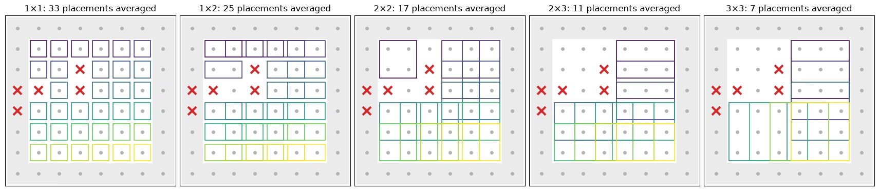
تعرض الخلية التالية المواضع من كل شكل التي تدخل في المتوسطات أدناه: كل موضع في صلب الشبكة دون موقع معلَّم (علامات × حمراء). أما المواضع التي تلامس الحافة (مظلَّلة) فتُستبعد. كيوبتات الحافة لها روابط أقل، فتتشوّش ببطء أكبر. وعند حساب متوسطها وحدها، تعبر نقطة التقاطع بخطوة كاملة من بعد مواضع الصلب، لكل شكل ولكل طريقة. ولكل موضع داخل في المتوسط صندوقه الخاص، ملوّن بحسب الموضع.
def touches_edge(qubits):
    # Whether a placement includes a site on the edge of the lattice
    return any(
        q % num_cols_hw in (0, num_cols_hw - 1)
        or q // num_cols_hw in (0, num_rows_hw - 1)
        for q in qubits
    )

# The placements of each shape that enter the averages: in the bulk, and without a flagged site
kept_placements = {
    label: [
        k
        for k, qubits in enumerate(patch_list)
        if not touches_edge(qubits) and not set(qubits) & flagged
    ]
    for label, patch_list in positions.items()
}
placement_cmap = plt.get_cmap("viridis")
fig, axes = plt.subplots(
    1, len(positions), figsize=(17, 4.4), layout="constrained"
)
for ax, (label, patch_list) in zip(axes, positions.items()):
    width, height = patch_shapes[label]
    for q in range(num_qubits_hw):
        x, y = q % num_cols_hw, q // num_cols_hw
        if touches_edge([q]):  # shade the edge of the lattice
            ax.add_patch(
                plt.Rectangle(
                    (x - 0.5, y - 0.5), 1, 1, color="0.92", zorder=0
                )
            )
        ax.plot(x, y, "o", color="0.7", ms=4, zorder=1)
    kept = kept_placements[label]
    for i, k in enumerate(kept):
        qubits = patch_list[k]
        x0, y0 = (
            qubits[0] % num_cols_hw,
            qubits[0] // num_cols_hw,
        )  # top-left site of the placement
        ax.add_patch(
            plt.Rectangle(
                (x0 - 0.4, y0 - 0.4),
                width - 0.2,
                height - 0.2,
                fill=False,
                lw=1.2,
                ec=placement_cmap(i / max(len(kept) - 1, 1)),
                zorder=2,
            )
        )
    for q in flagged:
        ax.plot(
            q % num_cols_hw,
            q // num_cols_hw,
            "x",
            color="#d62728",
            ms=11,
            mew=3,
            zorder=3,
        )
    ax.set_xlim(-0.6, num_cols_hw - 0.4)
    ax.set_ylim(num_rows_hw - 0.4, -0.6)
    ax.set_aspect("equal")
    ax.set_xticks([])
    ax.set_yticks([])
    ax.set_title(f"{label}: {len(kept)} placements averaged")
plt.show()
PEA
الطريقة الثالثة لا تحتاج إلى مرجع كلاسيكي. لكل تكافؤ، خذ القيم عند عوامل الضوضاء 1 و1.5 و2، واقسم على إخماد القراءة المتعلَّم (TREX)، ثم طابق دالة أسية في عامل الضوضاء، واستقرئ إلى انعدام الضوضاء. أما التكافؤات التي تغيّر إشارتها أو تقترب من الصفر فتُطابَق بخط مستقيم. يتطلب طرح التباين تقديرًا موثوقًا له، وهذا سهل للتكافؤات الخام والمُعاد تحجيمها لكنه ليس كذلك لمخرجات مطابقة غير خطية مع القص والحلول البديلة. لذلك تستخدم PEA الطريقة القياسية الأخرى لإزالة انحياز المربع: استقرئ كل نصف من العشوائيات على حدة، واضرب التقديرين المستقلين.
def readout_fidelity(support):
    # Damping of <Z_S> by the learned readout noise
    pauli = QubitSparsePauli.from_sparse_label(
        ("Z" * len(support), list(support)), num_qubits_hw
    )
    return readout_map.pauli_fidelity(pauli)

def extrapolate_to_zero(values):
    # Fit a * exp(b * factor) to each column of values (noise factors first), or a line
    # where the values change sign or come within 1e-3 of zero
    result = np.polynomial.polynomial.polyfit(noise_factors, values, 1)[0]
    sign = np.sign(values[0])
    usable = np.all(np.sign(values) == sign, axis=0) & (
        np.abs(values).min(axis=0) > 1e-3
    )
    if usable.any():
        log_fit = np.polynomial.polynomial.polyfit(
            noise_factors, np.log(np.abs(values[:, usable])), 1
        )
        result[usable] = sign[usable] * np.exp(log_fit[0])
    return result

def pea_ipr(parities, fidelities, num_patch):
    # parities has shape (noise factors, randomizations, supports). Extrapolate the two
    # halves of the randomizations separately; their errors are independent, so the
    # product of the two estimates of each parity has no shot-noise bias
    def zero_noise(p):
        # A parity cannot exceed 1 in magnitude, so cap the extrapolated values there
        return np.clip(
            extrapolate_to_zero(p.mean(axis=1) / fidelities), -1, 1
        )

    half = parities.shape[1] // 2
    first, second = (
        zero_noise(parities[:, :half]),
        zero_noise(parities[:, half:]),
    )
    return float((1 + np.dot(first, second)) / 2**num_patch)
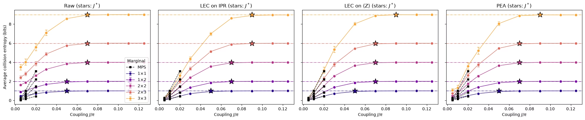
التقديرات الأربعة كلها ونقاط التقاطع
تحسب الدالة التالية التقديرات الخام، وLEC على IPR، وLEC على ، وPEA لـ IPR لموضع هامش واحد عند كل اقتران. كما تقدّر ضوضاء اللقطات لكل منها، بإعادة أخذ عينات العشوائيات (bootstrapping). تشغّلها الخلية لكل موضع داخل في المتوسطات، وهذا يستغرق نحو دقيقة ونصف.
def estimate_iprs(qubits, key):
    # Raw, LEC-on-IPR, LEC-on-<Z>, and PEA IPRs of one marginal position at every coupling,
    # with the shot noise of each from a bootstrap over the randomizations
    n = len(qubits)
    supports = parity_supports(qubits)
    # Parities with shape (noise factors, randomizations, supports), per coupling
    parities = [
        np.stack([parity_expectation_values(b, supports) for b in bits])
        for bits in raw_bits
    ]
    patch_bits = [
        bits[0][:, :, qubits] for bits in raw_bits
    ]  # noise factor 1
    values, errors = lec_estimates(
        patch_bits,
        [p[0] for p in parities],
        references[(calibration_hw, 64)][key],
        calibration_hw,
        n,
    )
    fidelities = np.array([readout_fidelity(s) for s in supports])

    def pea_statistic(p):
        return pea_ipr(p, fidelities, n)

    values["raw"] = [ipr_from_shots(b) for b in patch_bits]
    errors["raw"] = [bootstrap_error(ipr_from_shots, b) for b in patch_bits]
    values["PEA"] = [pea_statistic(p) for p in parities]
    errors["PEA"] = [
        bootstrap_error(pea_statistic, p, axis=1) for p in parities
    ]  # randomizations are axis 1
    return {m: np.array(v) for m, v in values.items()}, {
        m: np.array(e) for m, e in errors.items()
    }

methods = ["LEC on IPR", "LEC on ⟨Z⟩", "PEA"]
method_colors = {
    "LEC on IPR": "#2a78d6",
    "LEC on ⟨Z⟩": "#1baf7a",
    "PEA": "#eb6834",
}
iprs, ipr_errors = {}, {}
for label, patch_list in positions.items():
    for k in kept_placements[label]:
        iprs[label, k], ipr_errors[label, k] = estimate_iprs(
            patch_list[k], f"{label} {k}"
        )
print(f"{len(iprs)} clean marginal positions")
93 clean marginal positions
def crossover_coupling(couplings, entropies, haar, tolerance=0.1):
    # Smallest coupling whose entropy is within tolerance of the random-state value
    for coupling, entropy in zip(couplings, entropies):
        if entropy >= haar - tolerance:
            return coupling
    return None

def reference_ipr(index, chi, key):
    # IPR of the MPS distribution of a marginal
    return float((references[(index, chi)][key] ** 2).sum())

mps_settings = [
    (calibration_hw, 64),
    (1, 128),
    (2, 128),
]  # (coupling index, bond dimension)
panels = ["raw", *methods]

# Average IPR of every shape over its clean placements, then the entropy and the crossover
hw_entropies = {
    method: {} for method in panels
}  # per method and shape: average entropy and its error
crossovers = {method: {} for method in panels}
mps_entropies = {}  # per shape: MPS entropy, averaged over the same placements, at mps_settings
for label, patch_list in positions.items():
    haar = haar_entropy(len(patch_list[0]), num_qubits_hw)
    keys = [(shape, k) for (shape, k) in iprs if shape == label]
    mps_entropies[label] = [
        collision_entropy(
            np.mean([reference_ipr(j, chi, f"{label} {k}") for _, k in keys])
        )
        for j, chi in mps_settings
    ]
    for method in panels:
        ipr, ipr_error = average_ipr(
            [iprs[key][method] for key in keys],
            [ipr_errors[key][method] for key in keys],
        )
        entropy = collision_entropy(ipr)
        hw_entropies[method][label] = (entropy, ipr_error / (ipr * np.log(2)))
        crossovers[method][label] = crossover_coupling(
            couplings_hw, entropy, haar
        )
fig, axes = plt.subplots(
    1, len(panels), figsize=(5 * len(panels), 4.2), sharey=True
)
for (label, patch_list), color in zip(positions.items(), colors):
    haar = haar_entropy(len(patch_list[0]), num_qubits_hw)
    for ax, method in zip(axes, panels):
        entropy, error = hw_entropies[method][label]
        ax.errorbar(
            couplings_hw / np.pi,
            entropy,
            yerr=error,
            fmt="o-",
            color=color,
            mec="white",
            ms=7,
            lw=1,
            capsize=3,
            label=label,
        )
        ax.plot(
            couplings_hw[[j for j, _ in mps_settings]] / np.pi,
            mps_entropies[label],
            "s--",
            color="black",
            ms=4,
            lw=1,
            label="MPS" if label == "3×3" else None,
            zorder=4,
        )
        ax.axhline(haar, color=color, ls="dashdot", lw=0.9)
        if crossovers[method][label]:
            ax.plot(
                crossovers[method][label] / np.pi,
                haar,
                "*",
                ms=14,
                color=color,
                mec="black",
                zorder=3,
            )
for ax, method in zip(axes, panels):
    ax.set_title(f"{'Raw' if method == 'raw' else method} (stars: $J^*$)")
    ax.set_xlabel("Coupling $J/\\pi$")
axes[0].set_ylabel("Average collision entropy (bits)")
axes[0].legend(title="Marginal", loc="lower right")
fig.tight_layout()
plt.show()
الخلاصة
ما تطلّبه تشغيل تجربة بهذا الحجم:
-
دوائر لا تعتمد بنيتها على ، تُجمَّع طبقة فرعية في كل مرة، بحيث يخدم نموذج ضوضاء واحد المسح كله.
-
مقدِّرات تعمل من سلاسل البتات: عدّ الأزواج لحساب IPR لهامش، وصيغة Parseval، مع طرح التباين من كل تكافؤ مربّع، عندما تكون المدخلات قيمًا متوقعة مخففة.
-
مرساة كلاسيكية رخيصة: الحالة المثالية عند صغيرة تعاير الضوضاء، وتختبر الاقترانات المحجوزة المعايرة. ومعايرة كل على حدة، بدل IPR ككل، هي ما يجعل الهوامش الكبيرة تتفق.
-
أدوات IBM للأعمال الثقيلة: صناديق Samplomatic والتدوير العشوائي، و
NoiseLearnerV3، والفصل الديناميكي، ومهمةExecutorواحدة مع تضخيم الضوضاء لـ PEA. -
فحوصات جودة البيانات التي تستخدم البيانات فقط.
الخطوات التالية. لمزيد من التعمق في التخفيف، راجع الدرسين تضخيم الأخطاء الاحتمالي وPEC مع المخاريط الضوئية المظلَّلة.