التحسين الكمّي التقريبي متعدد الأهداف

تقدير الاستخدام: 10 دقائق على معالج Heron r2 (ملاحظة: هذا مجرد تقدير. قد يختلف وقت التشغيل لديك.)

مخرجات التعلّم

يحل هذا الدرس مسألة تحسين محفظة استثمارية مقيّدة بعدد الأصول: بالنظر إلى قيد الاحتفاظ بـ $K$ أصلًا بالضبط، نوازن بين أهداف المخاطرة والعائد والتنويع لإيجاد مجموعة المحافظ المثلى.

بعد إكمال هذا الدرس، يمكنك أن تتوقع أن تفهم:

• كيف تعبّر عن مسألة اختيار محفظة بثلاثة أهداف متنافسة — مخاطرة منخفضة وعائد مرتفع وتنويع جيد — كمسألة تحسين كمّي.

• كيف ترسم دائرة QAOA واحدة، تُمسح عبر مجموعة من أوزان الأهداف، جبهة Pareto للمحافظ المثلى ذات المفاضلة.

• كيف يُبقي XY mixer البحث داخل الفضاء الجزئي "اختيار K أصلًا بالضبط"، فلا حاجة إلى حد عقوبة، ويُفرض الاستيفاء بالانتقاء اللاحق لسلاسل البتات المقيسة.

• كيف تدرّب زوايا الدائرة باستخدام محاكي حالة حاصل ضرب المصفوفات بمقياس أكبر من أن يُحسَّن بدقة، وفقًا لـ Kotil وآخرين (arXiv:2503.22797).

المتطلبات المسبقة

يُنصح بأن تكون على دراية بـ:

• سير عمل أنماط Qiskit (التعيين، التحسين، التنفيذ، المعالجة اللاحقة).

• أساسيات QAOA.

الخلفية

نادرًا ما يحسّن مدير المحفظة رقمًا واحدًا. فهو يريد عوائد مرتفعة، ومخاطرة (تباين تلك العوائد) منخفضة، وحيازات موزعة على القطاعات حتى لا تتعرض المحفظة بإفراط لجزء واحد من السوق. هذه الأهداف تتعارض فيما بينها: فالأصول الأعلى عائدًا غالبًا ما تكون الأكثر تقلبًا، والتركيز في قطاع رائج واحد يضر بالتنويع.

لا توجد محفظة "أفضل" واحدة. بل توجد جبهة Pareto: مجموعة المحافظ التي لا يمكنك فيها تحسين هدف دون التخلي عن آخر. هدفنا هو رسم تلك الجبهة ليتمكن صانع القرار من اختيار المفاضلة التي يفضّلها.

نصوغ المسألة على أنها اختيار $K$ أصلًا بالضبط من بين $N$ (كل أصل إما داخل أو خارج — كيوبت واحد لكل أصل). ثلاثة هاملتونيات ترمّز الأهداف الثلاثة. ندمجها بأوزان $c$ تقع على simplex (مجموعها واحد)، ويعيد Sampler من نوع QAOA محافظ جيدة لكل اختيار للأوزان. مسح الأوزان يمسح الأهمية النسبية للمخاطرة مقابل العائد مقابل التنويع، ويرسم اتحاد كل المحافظ المأخوذة كعيّنات جبهة Pareto.

نستعرض أولًا سير العمل كاملًا على مثال صغير من ثمانية أصول يمكننا التحقق منه بالقوة الغاشمة، ثم نشغّل الطريقة نفسها على نسخة من 40 أصلًا بحجم مناسب للعتاد الكمّي.

يعلّم هذا الدرس سير العمل (التعيين، وتدريب الزوايا، وأخذ العيّنات المقيّد، والمعالجة اللاحقة لـ Pareto)، لا إظهار تفوق كمّي. عند مقياس الأصول الأربعين المستخدم هنا، يؤدي أخذ العيّنات العشوائي المنتظم بنفس مستوى Sampler من نوع QAOA تقريبًا، ونعرض هذه المقارنة صراحةً.

المتطلبات

قبل البدء في هذا الدرس، تأكد من تثبيت ما يلي:

• Qiskit SDK الإصدار 2.0 أو أحدث، مع دعم التصور

• Qiskit Runtime الإصدار 0.22 أو أحدث (pip install qiskit-ibm-runtime)

• Qiskit Aer (pip install qiskit-aer)

• إضافة Qiskit الخاصة بمُعيّن التحسين (pip install qiskit-addon-opt-mapper) وخط تدريب QAOA، مثبّتًا على الوسم v0.1.0: pip install "git+https://github.com/qiskit-community/qaoa_training_pipeline.git@v0.1.0"

• moocore لحسابات جبهة Pareto والحجم الفائق (pip install moocore)

الإعداد

استورد المكتبات المستخدمة طوال الدرس وثبّت بذرة عشوائية لإمكانية إعادة الإنتاج.

# Added by doQumentation — installs the packages this notebook needs if they are missing
import importlib.util

_needed = {"matplotlib": "matplotlib", "moocore": "moocore", "numpy": "numpy", "qaoa_training_pipeline": "qaoa-training-pipeline", "qiskit": "qiskit", "qiskit_addon_opt_mapper": "qiskit-addon-opt-mapper", "qiskit_aer": "qiskit-aer", "qiskit_ibm_runtime": "qiskit-ibm-runtime", "scipy": "scipy"}
_missing = [pip for module, pip in _needed.items()
            if importlib.util.find_spec(module) is None]
# One at a time, so a package that fails to install does not block the others
for _pip in _missing:
    %pip install -q {_pip}
if not _missing:
    print("\u2713 All required packages are installed")

import numpy as np
import matplotlib.pyplot as plt
from math import comb
from moocore import hypervolume, filter_dominated, is_nondominated

from qiskit import QuantumCircuit
from qiskit.circuit import ParameterVector
from qiskit.circuit.library import qaoa_ansatz
from qiskit.quantum_info import SparsePauliOp
from qiskit.transpiler import generate_preset_pass_manager
from qiskit_aer.primitives import SamplerV2 as AerSampler
from qiskit_addon_opt_mapper.problems import OptimizationProblem
from qaoa_training_pipeline.training import ScipyTrainer
from qaoa_training_pipeline.evaluation import (
    StatevectorEvaluator,
    MPSAerEvaluator,
)

np.random.seed(42)
sampler = AerSampler(seed=42)  # local simulator for the small-scale example
print("Setup complete.")

Setup complete.

مثال على محاكي صغير النطاق

نبدأ بثمانية أصول مأخوذة من ستة قطاعات ونختار $K=4$ منها بالضبط. مع ثمانية أصول فقط لا توجد إلا $\binom{8}{4}=70$ محفظة صالحة، لذا يمكننا لاحقًا مقارنة النتيجة الكمّية ببحث شامل.

الخطوة 1: تعيين المدخلات الكلاسيكية إلى مسألة كمّية

كل أصل هو كيوبت واحد؛ وسلسلة بتات مثل 10110010 هي محفظة (الأرقام 1 هي الأصول التي نحتفظ بها). نحتاج إلى ثلاثة مكوّنات: بيانات السوق، والهاملتونيات الثلاثة للأهداف، ودائرة لا تقترح إلا محافظ تحتوي على $K$ أصلًا بالضبط.

# --- Small-scale universe: 8 assets across 6 sectors ---
tickers = ["AAPL", "XOM", "JPM", "JNJ", "KO", "AMT", "AMZN", "SLB"]
sectors = [
    "Tech",
    "Energy",
    "Finance",
    "Health",
    "Staples",
    "REIT",
    "Tech",
    "Energy",
]
n_assets = len(tickers)
K = 4  # choose exactly K assets
n_obj = 3  # risk, return, diversification

# Annualized expected returns
mu = np.array([0.28, 0.12, 0.22, 0.05, 0.08, 0.10, 0.32, 0.15])

# Annualized covariance matrix (the "risk" model)
sigma = np.array(
    [
        [0.070, 0.010, 0.020, 0.008, 0.005, 0.012, 0.045, 0.011],
        [0.010, 0.065, 0.015, 0.006, 0.004, 0.008, 0.009, 0.050],
        [0.020, 0.015, 0.055, 0.010, 0.007, 0.015, 0.018, 0.014],
        [0.008, 0.006, 0.010, 0.030, 0.012, 0.009, 0.007, 0.005],
        [0.005, 0.004, 0.007, 0.012, 0.025, 0.006, 0.004, 0.003],
        [0.012, 0.008, 0.015, 0.009, 0.006, 0.045, 0.011, 0.007],
        [0.045, 0.009, 0.018, 0.007, 0.004, 0.011, 0.085, 0.010],
        [0.011, 0.050, 0.014, 0.005, 0.003, 0.007, 0.010, 0.072],
    ]
)

# Diversification score: number of cross-sector pairs in the portfolio.
# D[i,j] = 0.5 when assets i and j are in different sectors, so x^T D x counts
# the cross-sector pairs. More cross-sector pairs = better diversified.
D = np.array(
    [
        [1.0 if sectors[i] != sectors[j] else 0.0 for j in range(n_assets)]
        for i in range(n_assets)
    ]
)
np.fill_diagonal(D, 0.0)
D = D / 2

print(f"{n_assets} assets, choose K={K}, {n_obj} objectives")
for t, s, m in zip(tickers, sectors, mu):
    print(f"  {t:5s} ({s:8s})  expected return {m:5.0%}")

8 assets, choose K=4, 3 objectives
  AAPL  (Tech    )  expected return   28%
  XOM   (Energy  )  expected return   12%
  JPM   (Finance )  expected return   22%
  JNJ   (Health  )  expected return    5%
  KO    (Staples )  expected return    8%
  AMT   (REIT    )  expected return   10%
  AMZN  (Tech    )  expected return   32%
  SLB   (Energy  )  expected return   15%

# Each objective becomes a Hamiltonian whose lowest-energy bitstrings are the
# best portfolios for that objective. The opt-mapper turns a plain
# min/max problem over binary variables into the equivalent Ising operator.
def build_risk_hamiltonian(sigma, n):
    """Minimize portfolio variance x^T sigma x  (quadratic -> ZZ terms)."""
    prob = OptimizationProblem("risk")
    prob.binary_var_list(n)
    prob.minimize(quadratic=sigma)
    op, _ = prob.to_ising()
    return op.simplify()

def build_return_hamiltonian(mu, n):
    """Maximize expected return mu . x  (linear -> Z terms)."""
    prob = OptimizationProblem("return")
    prob.binary_var_list(n)
    prob.maximize(linear=mu)
    op, _ = prob.to_ising()
    return op.simplify()

def build_diversity_hamiltonian(D, n):
    """Maximize cross-sector pairs x^T D x  (quadratic -> ZZ terms)."""
    prob = OptimizationProblem("diversity")
    prob.binary_var_list(n)
    prob.maximize(quadratic=D)
    op, _ = prob.to_ising()
    return op.simplify()

H_risk = build_risk_hamiltonian(sigma, n_assets)
H_return = build_return_hamiltonian(mu, n_assets)
H_diversity = build_diversity_hamiltonian(D, n_assets)
cost_ops = [H_risk, H_return, H_diversity]

for name, op in zip(["risk", "return", "diversity"], cost_ops):
    print(f"H_{name:10s}: {op.size} Pauli terms")

H_risk      : 36 Pauli terms
H_return    : 8 Pauli terms
H_diversity : 34 Pauli terms

فرض "K أصلًا بالضبط" دون عقوبة. حيلة شائعة هي إضافة حد عقوبة يعاقب المحافظ ذات الحجم الخاطئ، لكنه يقرن كل كيوبت بكل كيوبت آخر، مما يؤدي إلى دوائر أعمق بكثير بعد transpile. بدلًا من ذلك نستخدم XY mixer، الذي لا يحرّك حالة QAOA إلا بين سلاسل البتات ذات وزن هامينغ نفسه. فإذا بدأنا من حالة فيها $K$ أصلًا مختارًا أصلًا، فإن كل محفظة تستكشفها الدائرة تحتوي أيضًا على $K$ أصلًا بالضبط. القيد مدمج في بنية الدائرة بدلًا من فرضه بحد عقوبة.

نحضّر الحالة الابتدائية بكلفة زهيدة: ندوّر كل كيوبت ليكون "مفعّلًا" باحتمال $K/N$. وعند الاقتصار على نتائج $K$ أصلًا، يُعيد هذا إنتاج حالة الأوزان المتساوية المثالية (حالة Dicke)، لذا نكتفي بإبقاء سلاسل البتات المقيسة التي تحتوي على $K$ من الآحاد بالضبط — خطوة تسمى الانتقاء اللاحق.

def xy_mixer(n):
    """Line XY mixer: couples neighboring qubits with XX+YY. Conserves the number
    of selected assets (Hamming weight), so cardinality is preserved automatically.
    Using a line (not a full ring) keeps the circuit shallow and hardware-friendly."""
    terms = [
        (pauli, [i, i + 1], 1) for i in range(n - 1) for pauli in ("XX", "YY")
    ]
    return SparsePauliOp.from_sparse_list(terms, n)

def product_init(n, k):
    """Cheap initial state: each qubit rotated so P(selected) = k/n. Zero two-qubit
    gates. Post-selecting its weight-k outcomes reproduces the ideal Dicke state."""
    qc = QuantumCircuit(n)
    theta = 2 * np.arcsin(np.sqrt(k / n))
    for q in range(n):
        qc.ry(theta, q)
    return qc

# Combine the three objectives with weights c (bound later, at sampling time).
p_layers = 1
c = ParameterVector("c", n_obj)
# Negate the objective so the sampling phase separator matches the sign the angles
# were trained under (the trainer maximizes the negated sum); binding below keeps +gamma.
combined_cost_op = sum(
    -c[k] * H_k for k, H_k in enumerate(cost_ops)
).simplify()

ansatz = qaoa_ansatz(
    combined_cost_op,
    reps=p_layers,
    initial_state=product_init(n_assets, K),
    mixer_operator=xy_mixer(n_assets),
)
ansatz.measure_all()

betas = [p for p in ansatz.parameters if p.name.startswith("β")]
gammas = [p for p in ansatz.parameters if p.name.startswith("γ")]
print(f"Qubits: {ansatz.num_qubits} | QAOA layers: {p_layers}")
print(
    f"Tunable angles: {len(betas)} beta + {len(gammas)} gamma, plus {n_obj} objective weights"
)

Qubits: 8 | QAOA layers: 1
Tunable angles: 1 beta + 1 gamma, plus 3 objective weights

الخطوة 2: تحسين المسألة للتنفيذ على العتاد الكمّي

قبل التشغيل، يُجرى transpile للدائرة المجردة إلى بوابات أصلية للعتاد. عند هذا المقياس الصغير نفحص الكلفة فقط: ما عمق الدائرة وكم عدد البوابات ثنائية الكيوبت التي تستخدمها؟ (البوابات ثنائية الكيوبت هي المصدر الرئيسي للضوضاء في الأجهزة الحقيقية.)

# Bind dummy angle values so we can transpile and measure the circuit's size.
dummy = {p: 0.1 for p in ansatz.parameters}
test_pm = generate_preset_pass_manager(optimization_level=1)
test_qc = test_pm.run(ansatz.assign_parameters(dummy))

print(f"Circuit depth          : {test_qc.depth()}")
print(
    f"Two-qubit gate depth   : {test_qc.depth(lambda x: len(x.qubits) > 1)}"
)
print(f"Two-qubit gate count   : {test_qc.num_nonlocal_gates()}")

Circuit depth          : 25
Two-qubit gate depth   : 23
Two-qubit gate count   : 42

الخطوة 3: التنفيذ باستخدام primitives الخاصة بـ Qiskit

مرحلتان. أولًا ندرّب زوايا QAOA مرة واحدة، باستخدام أوزان أهداف متساوية، مع محاكي متجه حالة دقيق لإيجاد قيم $\beta,\gamma$ جيدة. ثم نمسح متجهات أوزان كثيرة عبر simplex ونأخذ عيّنات من الدائرة عند كل منها، فنجمع محافظ مرشحة. ولأن أوزان الأهداف فقط هي التي تتغير بين عمليات المسح (لا الزوايا المدرَّبة)، تُرسل كل متجهات الأوزان في مهمة واحدة مجمّعة.

# Train the angles with equal objective weights.
# The trainer maximizes energy, so we negate the (to-be-minimized) objective sum.
training_op = sum(-1.0 / n_obj * H_k for H_k in cost_ops).simplify()

# Linear-ramp initialization (Sack and Serbyn, arXiv:2101.05742)
dt = 0.75
grid = np.arange(1, p_layers + 1) - 0.5
init_params = np.concatenate((1 - grid * dt / p_layers, grid * dt / p_layers))

trainer = ScipyTrainer(
    StatevectorEvaluator(), minimize_args={"options": {"maxiter": 300}}
)
print("Training QAOA angles (exact statevector)...")
result_train = trainer.train(
    cost_op=training_op,
    mixer=xy_mixer(n_assets),
    initial_state=product_init(n_assets, K),
    params0=init_params,
)
opt = result_train["optimized_params"]
opt_betas, opt_gammas = opt[:p_layers], opt[p_layers:]
print(f"Trained beta : {opt_betas}")
print(f"Trained gamma: {opt_gammas}")

Training QAOA angles (exact statevector)...
Trained beta : [3.329186967386619]
Trained gamma: [3.4449804324291033]

def random_uniform_simplex(n_samples, n_obj=3):
    """n_samples weight vectors spread uniformly over the (n_obj-1)-simplex."""
    s = np.zeros((n_samples, n_obj + 1))
    s[:, 1:-1] = np.random.rand(n_samples, n_obj - 1)
    s[:, -1] = 1
    s = np.sort(s, axis=1)
    return np.diff(s, axis=1)

# Bind the trained angles, leaving the objective weights c free for the sweep.
param_map = {betas[i]: opt_betas[i] for i in range(p_layers)}
param_map.update({gammas[i]: opt_gammas[i] for i in range(p_layers)})
ansatz_bound = ansatz.assign_parameters(param_map)

n_samples, shots = 200, 500
c_vecs = random_uniform_simplex(n_samples, n_obj)

print(f"Sampling {n_samples} weight vectors x {shots} shots...")
result = sampler.run([(ansatz_bound, c_vecs)], shots=shots).result()

# Collect every distinct bitstring seen across all weight vectors.
all_bitstrings = set()
for s in range(n_samples):
    for bs in result[0].data.meas.get_counts(s):
        # get_counts is little-endian; reverse so bit i = asset i
        all_bitstrings.add(bs.replace(" ", "")[::-1])
print(f"Distinct portfolios sampled: {len(all_bitstrings)}")

Sampling 200 weight vectors x 500 shots...
Distinct portfolios sampled: 256

الخطوة 4: المعالجة اللاحقة وإرجاع النتيجة بالصيغة الكلاسيكية المطلوبة

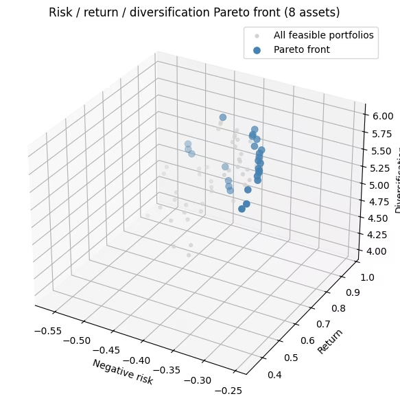
نحتفظ فقط بالمحافظ الممكنة (بالضبط $K$ من الأصول من خطوة الاختيار اللاحق)، ونقيّم كل واحدة منها وفق الأهداف الثلاثة كلها، ثم نستخرج جبهة باريتو: وهي المحافظ التي لا يتفوق عليها غيرها في كل الأهداف في الوقت نفسه. أما الحجم الفائق (hypervolume) فهو رقم واحد يلخّص مقدار فضاء الأهداف الذي تهيمن عليه الجبهة، وكلما كان أكبر كان أفضل.

مع 100,000 لقطة على 256 سلسلة بتات فقط، يرى هذا التشغيل كل المحافظ الصالحة السبعين، لذا فهو عند هذا الحجم فحص بالقوة الغاشمة فعليًا للتأكد من سلامة ربط خط المعالجة، لا دليلًا على أن QAOA وجد الجبهة.

def evaluate_portfolio(bitstring, sigma, mu, D):
    """Score one portfolio on all three objectives (all framed as 'bigger is better')."""
    x = np.array([int(b) for b in bitstring])
    # negative risk, return, diversification (cross-sector pairs)
    return np.array([-(x @ sigma @ x), x @ mu, x @ D @ x])

# Post-select feasible portfolios, then score them.
feasible = [bs for bs in all_bitstrings if bs.count("1") == K]
fis = np.array([evaluate_portfolio(bs, sigma, mu, D) for bs in feasible])

pareto_front = filter_dominated(fis, maximise=True)
ref_point = fis.min(axis=0)
qmoo_hv = hypervolume(fis, ref=ref_point, maximise=True)

print(
    f"Feasible portfolios found : {len(feasible)} of {comb(n_assets, K)} possible"
)
print(f"Pareto-front portfolios   : {len(pareto_front)}")
print(f"Hypervolume               : {qmoo_hv:.4f}")

Feasible portfolios found : 70 of 70 possible
Pareto-front portfolios   : 26
Hypervolume               : 0.2487

fig = plt.figure(figsize=(8, 6))
ax = fig.add_subplot(111, projection="3d")
ax.scatter(
    fis[:, 0],
    fis[:, 1],
    fis[:, 2],
    c="lightgray",
    s=12,
    label="All feasible portfolios",
)
ax.scatter(
    pareto_front[:, 0],
    pareto_front[:, 1],
    pareto_front[:, 2],
    c="steelblue",
    s=45,
    label="Pareto front",
)
ax.set_xlabel("Negative risk")
ax.set_ylabel("Return")
ax.set_zlabel("Diversification")
ax.set_title("Risk / return / diversification Pareto front (8 assets)")
ax.legend()
plt.tight_layout()
plt.show()

مثال على العتاد واسع النطاق

الآن سير العمل نفسه على 40 أصلًا (8 قطاعات × 5)، مع اختيار $K=6$. أربعون كيوبت أكبر من أن تُحاكى بدقة (متجه حالة بـ $2^{40}$ سعة)، لذا لا يمكن تحسين الزوايا بالطريقة نفسها كما في ثمانية أصول، وستكون الدائرة الكثيفة أعمق من أن يتحملها العتاد الحالي. أما $\binom{40}{6} \approx 3.8$M محفظة صالحة فلا تزال قليلة بما يكفي لتعدادها كلاسيكيًا، وهو ما نستخدمه في النهاية كمعيار دقيق. تتغير عدة أشياء، ولا شيء آخر في الطريقة يتغير:

1. درّب الزوايا باستخدام محاكي حالة حاصل ضرب المصفوفات (MPS)، لا متجه الحالة الدقيق. وفقًا للمرجع (Kotil وآخرون)، نثبّت أوزان الأهداف على قيم متساوية، ونحسّن β وγ واحدين على محاكي MPS، ونعيد استخدامهما لكل متجه أوزان في المسح. (ندرّب بالحجم الذي نشغّله — دون نقل زوايا من الصغير إلى الكبير.)

2. اجعل نموذج المخاطرة متناثرًا ليلائم العتاد. يقرن التباين المشترك الكامل كل أزواج الأصول البالغة 780. نُبقي فقط على الاقترانات الأقوى والأرخص توجيهًا باستخدام اقتطاع QAP الواعي بالأهمية، ونقرن كل قطاع في حلقة خفيفة لحد التنوع. هذا يُبقي الأهداف ذات معنى مع إبقاء الدائرة بحجم ملائم للعتاد.

3. أبقِ الدائرة ضحلة وقيّم بأمانة. التوجيه عشوائي، لذا نجري transpile بعدة بذور ونُبقي الأقل عمقًا (ولا يُستهلك أي وقت كمّي). تُقيَّم المحافظ دائمًا مقابل الأهداف الحقيقية الكاملة. التناثر يشكّل الدائرة فقط، لا طريقة الحكم على المحافظ.

لماذا اقتطاع QAP؟

قد يؤدي إبقاء أكبر اقترانات كل أصل بالمقدار وحده إلى دائرة متناثرة لكنها لا تزال صعبة التوجيه. أما اقتطاع QAP فيُبقي الاقترانات الكبيرة والقريبة فيزيائيًا على الشريحة معًا، فيشتري الميزان نفسه من البوابات دائرة أقل عمقًا وأكثر ملاءمة للعتاد.

الخطوة 1: تعيين المدخلات (متناثرة للعتاد)

import csv
import urllib.request

# Download the committed market-data snapshot from the repo.
# --- 40-asset universe: 8 GICS sectors x 5 tickers (real market data) ---
# Load the committed market-data snapshot (real annualized returns and covariance).
# Values are stored at the precision used to train the shipped QAOA angles
# (mu: 3 dp, sigma: 4 dp), so the pre-trained parameters in instances/ stay exactly valid.

url = "https://raw.githubusercontent.com/Qiskit/documentation/main/datasets/tutorials/qmoo/market_data.csv"
urllib.request.urlretrieve(url, "market_data.csv")

with open("market_data.csv", newline="") as _f:
    _rows = list(csv.reader(_f))

# Covariance column order
_tickers_csv = _rows[0][2:]
# Asset tickers
tickers_40 = [r[0] for r in _rows[1:]]
# Annualized expected returns
mu_40 = np.array([float(r[1]) for r in _rows[1:]])
# Covariance (risk model)
sigma_40 = np.array([[float(v) for v in r[2:]] for r in _rows[1:]])

sectors_40 = [
    "Tech",
    "Tech",
    "Tech",
    "Tech",
    "Tech",
    "Energy",
    "Energy",
    "Energy",
    "Energy",
    "Energy",
    "Finance",
    "Finance",
    "Finance",
    "Finance",
    "Finance",
    "Health",
    "Health",
    "Health",
    "Health",
    "Health",
    "Staples",
    "Staples",
    "Staples",
    "Staples",
    "Staples",
    "Industrials",
    "Industrials",
    "Industrials",
    "Industrials",
    "Industrials",
    "Utilities",
    "Utilities",
    "Utilities",
    "Utilities",
    "Utilities",
    "REIT",
    "REIT",
    "REIT",
    "REIT",
    "REIT",
]
n_assets_40 = len(tickers_40)
K_40 = 6  # choose exactly K assets

sector_names_40 = list(dict.fromkeys(sectors_40))
sect_idx_40 = np.array([sector_names_40.index(s) for s in sectors_40])
# True cross-sector diversification matrix (used for scoring)
D_40 = np.array(
    [
        [
            0.5 if sectors_40[i] != sectors_40[j] else 0.0
            for j in range(n_assets_40)
        ]
        for i in range(n_assets_40)
    ]
)
np.fill_diagonal(D_40, 0.0)
print(
    f"{n_assets_40} assets, {len(sector_names_40)} sectors, choose K={K_40}"
)

40 assets, 8 sectors, choose K=6

# Sparsify the covariance so the risk circuit fits on hardware. A small diagonal
# shift (added after truncation) keeps the risk model positive semidefinite; at fixed
# K it adds the same constant to every portfolio, so it never changes the ranking.
# Importance-aware QAP truncation (Kotil et al. style): place the qubits on a line
# and use a Quadratic Assignment Problem to choose the layout that keeps the
# strongest covariance couplings within routing distance k of the swap network,
# then drop the rest. Unlike a fixed top-k cap, it keeps couplings that are both
# large AND cheap to route.
from scipy.optimize import quadratic_assignment as qap
from qiskit.transpiler.passes.routing.commuting_2q_gate_routing import (
    SwapStrategy,
)

# Truncation level: larger k keeps more couplings (deeper circuit)
k_truncate = 2
_dist = np.array(
    SwapStrategy.from_line(list(range(n_assets_40))).distance_matrix
)

def qap_truncate(Q, k):
    w = np.abs(Q.copy())
    np.fill_diagonal(w, 0.0)
    mask = (_dist <= k).astype(float)
    # Seed the QAP solver explicitly (by default it draws from NumPy's global
    # RNG, which SciPy is deprecating) so the truncation is reproducible.
    perm = qap(-w, mask, options={"rng": np.random.default_rng(42)}).col_ind
    keep = mask[np.ix_(perm, perm)]
    Qt = Q * keep
    np.fill_diagonal(Qt, np.diag(Q))
    return Qt

sigma_sparse = qap_truncate(sigma_40, k_truncate)
print(
    f"QAP truncation (k={k_truncate}): risk edges kept = "
    f"{(np.count_nonzero(sigma_sparse) - n_assets_40) // 2}"
)
ridge = max(0.0, -np.linalg.eigvalsh(sigma_sparse)[0]) + 1e-6
sigma_sparse = sigma_sparse + ridge * np.eye(n_assets_40)

# Diversity: couple each sector's assets in a ring (sparse stand-in for the
# same-sector pair count). Scoring still uses the true cross-sector matrix D_40.
def build_same_sector_hamiltonian(D_same, n):
    prob = OptimizationProblem("diversity_sparse")
    prob.binary_var_list(n)
    prob.minimize(quadratic=D_same)
    op, _ = prob.to_ising()
    return op.simplify()

D_ring = np.zeros((n_assets_40, n_assets_40))
for s in set(sect_idx_40):
    members = np.where(sect_idx_40 == s)[0]
    for k in range(len(members)):
        i, j = members[k], members[(k + 1) % len(members)]
        D_ring[i, j] = D_ring[j, i] = 0.5

H_risk_40 = build_risk_hamiltonian(sigma_sparse, n_assets_40)
H_return_40 = build_return_hamiltonian(mu_40, n_assets_40)
H_diversity_40 = build_same_sector_hamiltonian(D_ring, n_assets_40)
cost_ops_40 = [H_risk_40, H_return_40, H_diversity_40]
n_zz = sum(
    1 for p in sum(cost_ops_40).simplify().paulis if str(p).count("Z") == 2
)
print(
    f"Cost-layer interactions: {n_zz} (dense would be {n_assets_40*(n_assets_40-1)//2})"
)

QAP truncation (k=2): risk edges kept = 78
Cost-layer interactions: 102 (dense would be 780)

الخطوتان 2-3: تدريب الزوايا، ثم بناء مهمة العتاد وإرسالها

أربعون كيوبت أكبر من أن تُحسَّن الزوايا فيها بدقة، لذا ندرّب $\beta, \gamma$ واحدين على محاكي حالة حاصل ضرب المصفوفات بأوزان أهداف متساوية ونعيد استخدامهما عبر المسح. تحمّل الخلية أدناه قيمًا مدرَّبة مسبقًا من ملف. زاوية طبقة الكلفة المدرَّبة صغيرة ($\gamma \approx 0.32$)، لذا تطبّق الدائرة انحيازًا لطيفًا بدلًا من إسقاط حاد.

import json
from qiskit_ibm_runtime import QiskitRuntimeService, SamplerV2

# Pre-trained angles loaded from a file (training is slow; QDC pattern).
# Set load_params_file = False to retrain in-notebook.
load_params_file = True
params_url = "https://raw.githubusercontent.com/Qiskit/documentation/main/datasets/tutorials/qmoo/qaoa_params.json"
params_path = "qaoa_params.json"
if load_params_file:
    urllib.request.urlretrieve(params_url, params_path)
    qaoa_params = json.load(open(params_path))
    p_layers_hw = qaoa_params["p_layers"]
    opt_betas_40, opt_gammas_40 = qaoa_params["betas"], qaoa_params["gammas"]
else:
    # Same workflow as the small-scale example: qaoa_training_pipeline's MPSAerEvaluator
    # evaluates the QAOA energy on Aer's MPS simulator and supports the XY mixer.
    # As in the small-scale example the trainer maximizes energy, so we negate the
    # (to-be-minimized) objective sum; the 1/n_obj scaling matches the equal-weight
    # point of the sweep, so the trained gamma transfers directly to the weighted circuits.
    p_layers_hw = 1
    training_op_40 = sum(-1.0 / n_obj * H_k for H_k in cost_ops_40).simplify()

    dt = 0.75
    grid = np.arange(1, p_layers_hw + 1) - 0.5
    init_params_40 = np.concatenate(
        (1 - grid * dt / p_layers_hw, grid * dt / p_layers_hw)
    )

    trainer_40 = ScipyTrainer(
        MPSAerEvaluator({"matrix_product_state_max_bond_dimension": 24}),
        minimize_args={"options": {"maxiter": 80}},
    )
    print("Training QAOA angles (MPS simulator)...")
    result_train_40 = trainer_40.train(
        cost_op=training_op_40,
        mixer=xy_mixer(n_assets_40),
        initial_state=product_init(n_assets_40, K_40),
        params0=init_params_40,
    )
    opt_40 = result_train_40["optimized_params"]
    opt_betas_40, opt_gammas_40 = (
        list(opt_40[:p_layers_hw]),
        list(opt_40[p_layers_hw:]),
    )
    import os

    os.makedirs(os.path.dirname(params_path) or ".", exist_ok=True)
    json.dump(
        {
            "p_layers": p_layers_hw,
            "betas": opt_betas_40,
            "gammas": opt_gammas_40,
        },
        open(params_path, "w"),
        indent=2,
    )
    print(
        f"Trained angles saved to {params_path} (set load_params_file=True to reuse)."
    )

c40 = ParameterVector("c", n_obj)
# Negated to match the trained angles' sign, as in the small-scale cell; binding keeps +gamma.
combined_cost_op_40 = sum(
    -c40[k] * H_k for k, H_k in enumerate(cost_ops_40)
).simplify()
qc_40 = qaoa_ansatz(
    combined_cost_op_40,
    reps=p_layers_hw,
    initial_state=product_init(n_assets_40, K_40),
    mixer_operator=xy_mixer(n_assets_40),
)
qc_40.measure_all()
b40 = [p for p in qc_40.parameters if p.name.startswith("β")]
g40 = [p for p in qc_40.parameters if p.name.startswith("γ")]
pmap = {b40[i]: opt_betas_40[i] for i in range(p_layers_hw)}
pmap.update({g40[i]: opt_gammas_40[i] for i in range(p_layers_hw)})
ansatz_qc_40 = qc_40.assign_parameters(pmap)

service = QiskitRuntimeService()

# only use Heron devices
backend = service.least_busy(min_num_qubits=156)

# SABRE routing is stochastic: different seeds give different depths. Transpilation
# is classical (it costs no QPU time), so we transpile many seeds and keep only the
# shallowest circuit -- a free reduction in two-qubit depth before anything is sent
# to hardware. Only this single best circuit is ever executed.
n_seeds = 24
best = None
depths = []
for seed in range(n_seeds):
    pm = generate_preset_pass_manager(
        optimization_level=3, backend=backend, seed_transpiler=seed
    )
    qc = pm.run(ansatz_qc_40)
    d2 = qc.depth(lambda x: len(x.qubits) > 1)
    depths.append(d2)
    if best is None or d2 < best[0]:
        best = (d2, seed, qc)
isa_qc = best[2]
sd = sorted(depths)
print(
    f"Backend: {backend.name} | {n_seeds} seeds | two-qubit depth "
    f"best/median/worst = {sd[0]}/{sd[len(sd)//2]}/{sd[-1]} (best seed {best[1]})"
)
print(
    f"Selected circuit -> two-qubit gates: {isa_qc.num_nonlocal_gates()}, "
    f"two-qubit depth: {isa_qc.depth(lambda x: len(x.qubits) > 1)}"
)

Backend: ibm_kingston | 24 seeds | two-qubit depth best/median/worst = 220/261/300 (best seed 22)
Selected circuit -> two-qubit gates: 787, two-qubit depth: 220

# Submit one batched job (job mode; a single batch needs no Session).
# Extra shots: noise lowers the post-selection yield
n_samples_40, shots_40 = 24, 1500
c_vecs_40 = random_uniform_simplex(n_samples_40, n_obj)
sampler_hw = SamplerV2(mode=backend)
# Tag hardware jobs for tracking
sampler_hw.options.environment.job_tags = ["TUT_QAMOO"]
# Seconds; guard against runaway jobs
sampler_hw.options.max_execution_time = 600

# The QAOA angles are already bound; only the objective weights c remain free.
# Assign each weight vector to get one concrete circuit per point on the simplex.
bound_circuits_40 = [
    isa_qc.assign_parameters({c40[k]: cv[k] for k in range(n_obj)})
    for cv in c_vecs_40
]
job_hw = sampler_hw.run([(qc,) for qc in bound_circuits_40], shots=shots_40)
print(
    f"Submitted to {backend.name}: job id {job_hw.job_id()} ({len(bound_circuits_40)} circuits)"
)

Submitted to ibm_kingston: job id darcaalvr3kc73einokg (24 circuits)

الخطوة 4: المعالجة اللاحقة إلى جبهة Pareto وقراءة المحافظ المثلى

result_hw = job_hw.result()

# Post-select feasible portfolios (exactly K assets), score on the TRUE objectives.
feasible_40 = set()
for s in range(n_samples_40):
    for bs in result_hw[s].data.meas.get_counts():
        # get_counts is little-endian; reverse so bit i = asset i
        bs = bs.replace(" ", "")[::-1]
        if bs.count("1") == K_40:
            feasible_40.add(bs)

def score_40(P):
    """Score portfolios given as an (n, K) array of asset indices.

    Returns an (n, 3) array of [negative risk, return, diversification], all framed
    as 'bigger is better'. This is the single definition of the true objectives,
    used for the hardware samples, the exact enumeration, and the random baseline.
    Looping over the K x K index pairs keeps memory O(n) even for millions of rows.
    """
    risk = np.zeros(len(P))
    div = np.zeros(len(P))
    for a in range(P.shape[1]):
        for b in range(P.shape[1]):
            risk += sigma_40[P[:, a], P[:, b]]
            div += D_40[P[:, a], P[:, b]]
    return np.column_stack([-risk, mu_40[P].sum(1), div])

def evaluate_40(bs):
    """Score one bitstring (bit i = asset i) with score_40."""
    idx = np.flatnonzero([b == "1" for b in bs])
    return score_40(idx[None, :])[0]

fis_40 = np.array([evaluate_40(bs) for bs in feasible_40])
pareto_40 = filter_dominated(fis_40, maximise=True)
print(f"Feasible portfolios collected : {len(feasible_40)}")
print(f"Pareto-front portfolios       : {len(pareto_40)}")

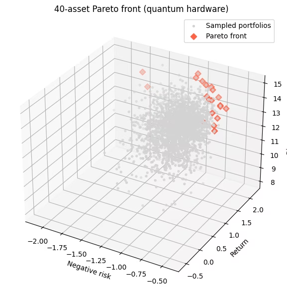
Feasible portfolios collected : 2359
Pareto-front portfolios       : 20

# --- Honest benchmark: QAOA and random vs the EXACT Pareto front ---
# 40 choose 6 = 3,838,380 feasible portfolios -- few enough to enumerate exactly, score
# every one on the TRUE objectives, and get the exact Pareto front. That front is an
# absolute ceiling, and its feasible nadir is a FIXED hypervolume reference point, so the
# numbers are comparable across runs instead of depending on what happened to be sampled.
import itertools

# Stream the combinations straight into an (n, K) index array, without first
# building millions of Python tuples.
combos = np.fromiter(
    itertools.chain.from_iterable(
        itertools.combinations(range(n_assets_40), K_40)
    ),
    dtype=np.int16,
).reshape(-1, K_40)
fis_exact = score_40(combos)
front_exact = filter_dominated(fis_exact, maximise=True)

# Fixed reference = worst value of each objective over ALL feasible portfolios (the nadir).
ref_fixed = fis_exact.min(axis=0)
# The hypervolume of a point set equals the hypervolume of its front.
hv_ceiling = hypervolume(front_exact, ref=ref_fixed, maximise=True)
hv_qaoa = hypervolume(fis_40, ref=ref_fixed, maximise=True)

def random_feasible_hv(n_draw, seed):
    """Hypervolume of n_draw uniformly-random feasible portfolios, same fixed reference."""
    rng = np.random.default_rng(seed)
    picks = set()
    while len(picks) < n_draw:
        picks.add(tuple(sorted(rng.choice(n_assets_40, K_40, replace=False))))
    P = np.array(list(picks))
    return hypervolume(score_40(P), ref=ref_fixed, maximise=True)

hv_rand = np.array(
    [random_feasible_hv(len(feasible_40), seed) for seed in range(20)]
)

print(f"Exact Pareto front            : {len(front_exact)} portfolios")
print(f"Hypervolume ceiling (optimum) : {hv_ceiling:.3f}")
print(
    f"QAOA (hardware)               : {100 * hv_qaoa / hv_ceiling:5.1f}% of optimum"
)
print(
    f"Random ({len(feasible_40)} draws, 20 seeds) : "
    f"{100 * hv_rand.mean() / hv_ceiling:5.1f}% +/- {100 * hv_rand.std() / hv_ceiling:.1f}% of optimum"
)

Exact Pareto front            : 61 portfolios
Hypervolume ceiling (optimum) : 64.211
QAOA (hardware)               :  85.5% of optimum
Random (2359 draws, 20 seeds) :  84.4% +/- 1.3% of optimum

عند حجم المسألة هذا، يؤدي QAOA بنفس مستوى أخذ العيّنات العشوائي المنتظم تقريبًا. كلاهما يستعيد جزءًا كبيرًا من الحجم الفائق للأمثل الدقيق، ولا أحد منهما متقدم بوضوح. هذه النتيجة متوقعة لطبقة QAOA ضحلة واحدة مع معامل كلفة مقتطع بشدة على عتاد مشوش؛ قيمة هذا المثال هي سير العمل متعدد الأهداف من البداية إلى النهاية (التعيين، وتدريب الزوايا، وأخذ العيّنات المقيّد، والمعالجة اللاحقة لـ Pareto)، لا تسريع كمّي. وتضييق الفجوة مع الأمثل يتطلب دوائر أعمق (طبقات QAOA أكثر)، أو اقتطاعًا ألطف، أو عتادًا أقل ضوضاء.

# The best trade-offs found by the sampler: no other sampled portfolio beats these
# on every objective. They approximate the exact front computed above; a
# decision-maker picks the trade-off they prefer.
bs_list = list(feasible_40)
# Boolean mask over fis_40; keep_weakly=True also keeps portfolios whose
# objective values tie with a front point (what the strict filter would drop).
mask = is_nondominated(fis_40, maximise=True, keep_weakly=True)
front_bs = [b for b, m in zip(bs_list, mask) if m]
front_f = fis_40[mask]
order = np.argsort(-front_f[:, 1])  # show a span sorted by return
print(
    f"{mask.sum()} non-dominated sampled portfolios. A representative span:\n"
)
print(
    f"{'tickers held':40s} {'risk':>7s} {'return':>7s} {'cross-sector':>12s}"
)
for idx in order[:: max(1, len(order) // 12)]:
    held = [tickers_40[i] for i, b in enumerate(front_bs[idx]) if b == "1"]
    print(
        f"{', '.join(held):40s} {-front_f[idx,0]:7.3f} {front_f[idx,1]:7.2f} {int(front_f[idx,2]):12d}"
    )

fig = plt.figure(figsize=(8, 6))
ax = fig.add_subplot(111, projection="3d")
ax.scatter(
    fis_40[:, 0],
    fis_40[:, 1],
    fis_40[:, 2],
    c="lightgray",
    s=8,
    label="Sampled portfolios",
)
ax.scatter(
    pareto_40[:, 0],
    pareto_40[:, 1],
    pareto_40[:, 2],
    c="tomato",
    marker="D",
    s=40,
    label="Pareto front",
)
ax.set_xlabel("Negative risk")
ax.set_ylabel("Return")
ax.set_zlabel("Diversification")
ax.set_title("40-asset Pareto front (quantum hardware)")
ax.legend()
plt.tight_layout()
plt.show()

20 non-dominated sampled portfolios. A representative span:

tickers held                                risk  return cross-sector
AAPL, NVDA, XOM, GS, BLK, CAT              1.715    2.22           13
NVDA, GS, MS, PFE, CAT, PLD                1.772    2.20           14
NVDA, MS, PFE, WMT, CAT, DUK               1.040    2.14           15
NVDA, CVX, GS, JNJ, KO, WMT                0.737    2.01           14
NVDA, COP, GS, JNJ, WMT, EQIX              1.014    1.98           15
NVDA, ABT, WMT, CAT, AEP, EQIX             0.913    1.92           15
NVDA, CVX, WMT, RTX, D, EQIX               0.835    1.82           15
NVDA, XOM, GS, JNJ, DUK, EQIX              0.763    1.80           15
AAPL, NVDA, JNJ, KO, RTX, SO               0.621    1.71           14
NVDA, CVX, BLK, JNJ, RTX, AEP              0.719    1.71           15
NVDA, JNJ, KO, COST, RTX, AEP              0.545    1.69           14
NVDA, CVX, ABT, WMT, HON, AEP              0.702    1.43           15
AAPL, GS, JNJ, PEP, AEP, EQIX              0.645    1.34           15
MSFT, XOM, BLK, JNJ, CAT, SO               0.617    1.34           15
MSFT, KO, WMT, RTX, SO, SPG                0.526    1.29           14
MSFT, XOM, BLK, JNJ, WMT, DUK              0.483    1.25           15
MSFT, CVX, JNJ, RTX, DUK, D                0.482    1.02           14
MSFT, XOM, JNJ, KO, HON, EQIX              0.479    0.93           15
MSFT, JNJ, PG, KO, RTX, DUK                0.423    0.86           14
MSFT, XOM, JNJ, PEP, DUK, AMT              0.476    0.57           15

الخطوات التالية

توصيات

إذا وجدت هذا الدرس مثيرًا للاهتمام، ففكّر فيما يلي:

• استبدل بيانات السوق المنزّلة (market_data.csv) بعوائدك وتقديرات التباين المشترك الخاصة بك من تاريخ أسعار حقيقي.

• زد عدد طبقات QAOA، أو درّب على 12–16 أصلًا وانقل تلك الزوايا، لتقريب جبهة العتاد من الأمثل.

• اقرأ Kotil وآخرون، Quantum Approximate Multi-Objective Optimization (Nature Computational Science، 2025)، دراسة max-cut التي يكيّفها هذا الدرس مع المحافظ.

المراجع

1. Kotil et al., "Quantum Approximate Multi-Objective Optimization," Nature Computational Science (2025). arXiv:2503.22797

2. S. H. Sack and M. Serbyn, "Quantum annealing initialization of the quantum approximate optimization algorithm," Quantum 5, 491 (2021). arXiv:2101.05742